I built my first and last Tesla coil 27 years ago in eighth grade. It won third place in the Illinois state science fair for my age group. I have recently become interested in Tesla coils again. I look forward to building my first coil since junior high school.
I use a circuit simulation program called PSpice in my day-to-day work as an electronics engineer. Personal Spice runs on PC's and Macs. PSpice allows you to use your computer as an electronic breadboard and oscilloscope. It will permit you to see the voltage wave forms at each circuit node or the current through each component. A circuit node is any point where two or more circuit components come together. PSpice saves you from difficult and tedious hand calculation, letting you be more creative.
Spice is a general purpose circuit simulation program developed at the University of California, Berkeley. Spice performs nonlinear DC, nonlinear transient (voltage vs time), and linear AC analysis. Circuits simulated may contain resistors, capacitors, inductors, mutual inductors, transmission lines, and the four most common semiconductor devices: diodes, BJTs, JFETs and MOSFETs. Circuit forcing functions are implemented by independent and four types of dependent voltage and current sources.
Features include:
- Simulation of electronic circuits
- Flexibility to change designs and test new ideas
- Component part tolerance checks and reports
- Check circuit ideas before breadboarding
- Try out ideal operation by using ideal components to isolate limiting effects in a design
- Simulate test measurements that are;
Difficult (due to electrical interference)
Inconvenient (special test equipment is unavailable)
Unwise (test circuit would destroy itself).
We will be using the evaluation version of PSpice. The evaluation version limits simulated circuits to ten transistors and about 20 circuit nodes. A package containing the evaluation version of PSpice, the current PSpice manual, and the book A Guide to Circuit Simulation & Analysis Using PSpice is available for $70 from MicroSim Corp, 20 Fairbanks, Irvine, CA 92718. The program is available on many bulletin boards.
To help with the design of a new coil I purchased some books on Tesla coil theory from High Energy Enterprises. The following analysis is of a 70 KV Tesla coil described in one of the books.
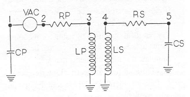
The schematic of the coil is shown in Figure 1, the PSpice input file is:
Tesla coil frequency response
CP
1
0
0.002U
.
RP
2
3
.03
.
LP
3
0
29.06U
.
LS
4
0
4.22M
.
RS
4
5
9.77
.
CS
5
0
13.77P
.
VAC
1
2
AC
1
K1
LP
LS
.25
.
.AC
LIN
2001
100000
2000000
.PROBE
.
.
.
.
.END
.
.
.
.
Figure 1.
The first line is a title line. Up to eighty characters are allowed. Each one of the lines following the title line describes a circuit element. The second line informs PSpice that capacitor CP connects from node one to node zero. CP has a value of 0.002 micro-farads. Node zero is reserved for ground. VAC is an ideal voltage source used in place of the spark gap to drive the Tesla coil. The line that begins .AC is a command line. It sweeps all AC voltage or current sources from 100,000Hz to 2,000,000Hz in 2,001 linear steps. The PROBE line saves the circuit node voltages and component currents into a disk file for later graphical analysis. The .END line denotes the end of the file.
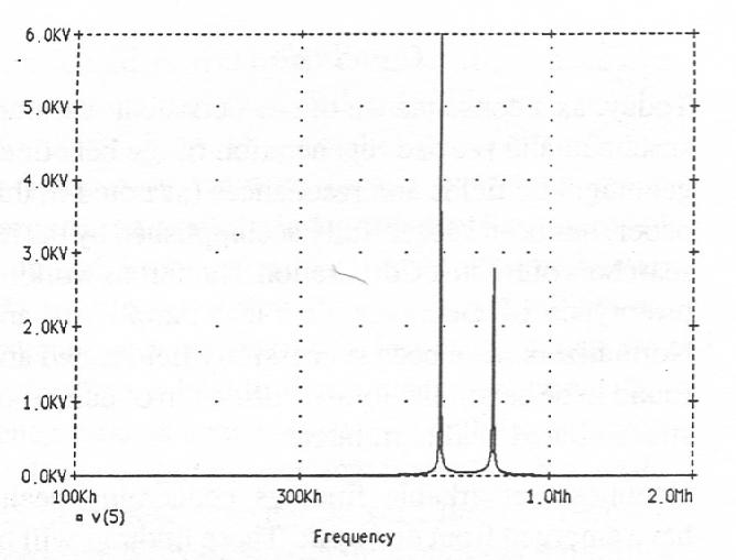
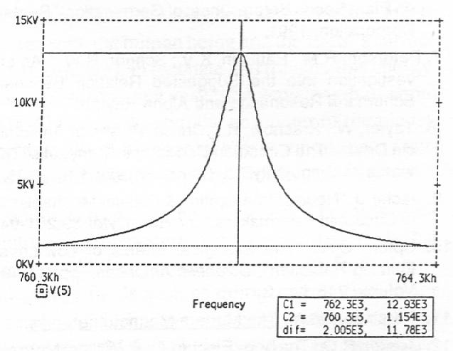
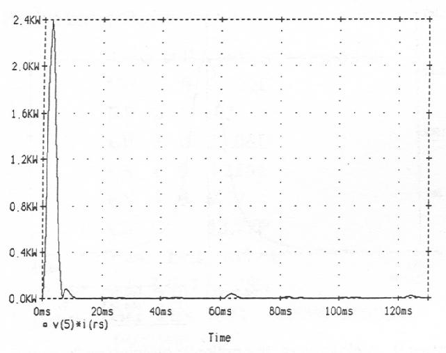
Figure 2. An overcoupled tuned resonant transformer.
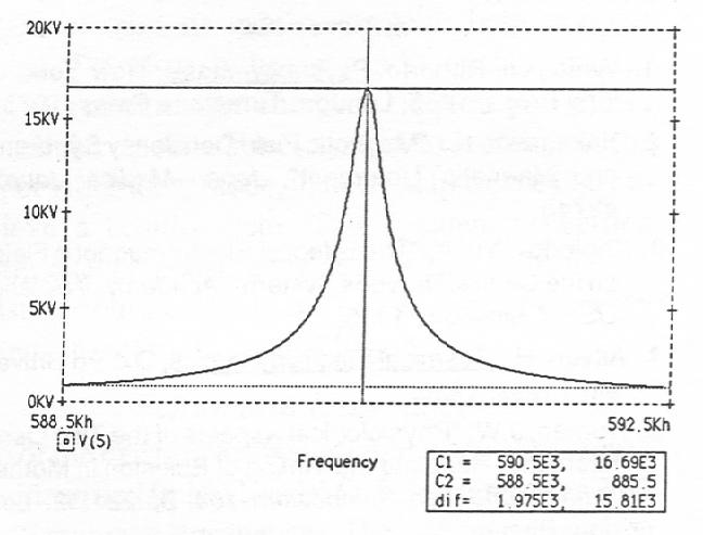
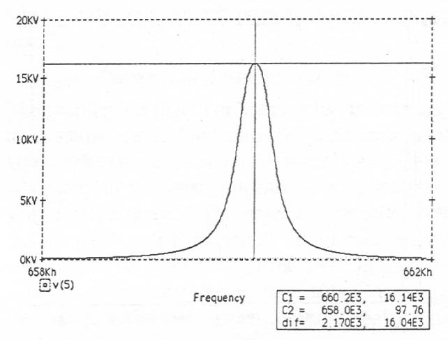
Figure 3. Close up of the left spike in Figure 2.
Figure 4. Close up of the right spike on Figure 2.
The line that begins with K1 defines the coupling coefficient between inductors LP and LS. I chose 0.25 because the book states that the coupling of these size Tesla coils has traditionally been between 0.2 and 0.3. When I ran PSpice using this input file, the Tesla coil output, node 5, looks like Figure 2.
The waveform in Figure 2 exhibits over coupling of a tuned resonant transformer. Figure 2 does not tell the whole story. The Probe output file cannot be larger than 150 Kilobytes and run properly with the evaluation version of PSpice. This necessitates a coarse frequency sweep for the large frequency range. The left-most spike is shown in greater detail in Figure 3. Figure 3 shows the output at Node 5 sampled every 5Hz. Figure 4 shows similar data for the right-most spike.
The skirts of the spikes are rather broad, indicating a lack of monochromaticity in the output. The two strong fundamentals, along with the mix of frequencies indicated by the broad skirts, will form beats. The output will have variations in amplitude due to the constructive and destructive summing of the output waveforms in the secondary. The output will sputter, running in pulses. Additionally, the beating of the two fundamental frequencies will form standing waves along the secondary. These standing waves will generate a nonuniform voltage distribution along the secondary coil. This can cause arcing from winding to winding on the secondary, eventually leading to its destruction.
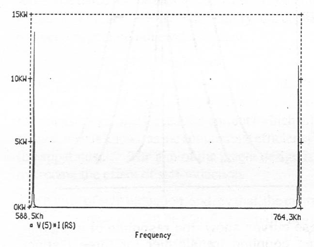
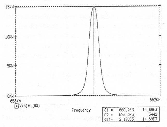
Figure 5. Power spectrum of the secondary circuit.
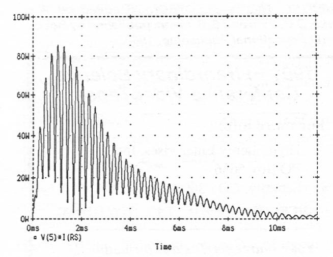
Figure 6. Fourier analysis of Figure 5.
Figure 7. Output of critically coupled coil.
Figure 8. A closeup of the critically coupled coil's peak.
Figure 5 shows the power in the secondary circuit over the frequency range of 588,500 Hz to 764,300 Hz sampled every 50 Hz. The X-axis is frequency. A Fourier analysis of the waveform in Figure 5 will transform the X-axis to time. Figure 6 shows the Fourier analysis of Figure 5. The area under the curve of Figure 6 is Watt-Seconds, or energy. The many humps in the curve are due to the beating of the two fundamental frequencies against one another. If we approximate the envelope of the curve with triangles, the energy comes out somewhere between 0.25 and 0.75 Watt-Seconds.
Critical coupling of a Tesla coil's primary and secondary inductors produce monochromatic output.
Figure 9. Power spectrum of critically coupled coil.
Figure 10. Fourier transform of power spectrum.
Critical coupling takes place when the coupling coefficient is equal to the reciprocal of the square root of the product of the quality factors of the two inductors.
The Q of the primary is 4477 and the secondary 1792. The coupling coefficient at critical coupling is 0.0003531. Figure 7 displays the output of the Tesla coil with the coupling coefficient set to 0.0003531. The output is one strong peak at a single frequency.
Figure 8 shows a close-up of the peak. Notice that the amplitude is greater than either of the two peaks in the previous example. The waveform has a sharper fall off and the skirts are lower in amplitude. This indicates a high degree of monochromaticity in the output.
Figure 9 shows the power contained in the peak of Figure 8. Figure 10, the Fourier transform of Figure 9, is most revealing! The energy contained in the secondary of this Tesla coil with a coupling coefficient of 0.0003531 is 6 Watt-Seconds. Wow!!!!
Proper coupling of the primary and secondary results in an energy output that is ten times greater than what traditional Tesla coil building techniques can achieve.
Traditional tuning of Tesla coils involves changing taps on the primary coil or adjusting the primary capacitance. This only fine tunes the Tesla coils frequency of operation. When I build my next Tesla coil I will mount the secondary on a jack screw. Changing the geometry allows fine tuning of the primary to secondary inductive coupling. I will report on my results in the future.
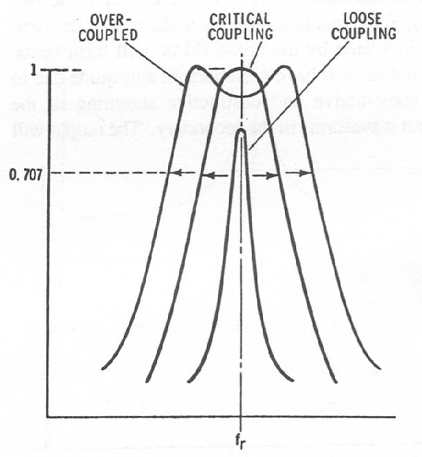
The Three Degrees of Coupling
These curves show the response of a double-tuned coupling transformer for three distinct degrees of coupling.
CREDITS: This is ELECTRONICS edited by W.E. Burke, D.G. Irvin and G.B. Mann, published by Bobbs-Merrill Educational Publishing, 1980.
Downloads
Downloads for this article are available to members. Log in or join today to access all content.
Downloads
Downloads for this article are available to members. Log in or join today to access all content.