Results of a prior experiment and its conclusions are re-examined by two researchers. Charge deposition on isolated capacities due to rapid discharge of "non-sparking" Tesla coils is tested a second time using a number of different techniques and instruments. This new, joint effort contradicts the prior work. Explanations are given as to why the prior conclusions were found to be in error.
A Simple Demonstration of Charge Deposition
The purpose of the first experiments was to examine in a most general but confirming manner the net deposition of charge from a pulsed Tesla coil to any nearby isotropic capacitance. The Tesla coil emits no spark nor corona in these tests and is discharged at a rate of one pulse per second.
To demonstrate, Richard Hull employed a dc supply of precisely 6 kilovolts to charge a 0.01 uf capacitor. This charged capacitor was then switched via a high power hydrogen thyratron across the primary of a Tesla coil. (See "The Hydrogen Thyratron" sidebar.) The secondary was a top loaded resonator that oscillated at 640 kHz. The very short, unidirectional current pulse to the primary turned off the hydrogen thyratron at zero crossing, thus opening the primary circuit, which then allowed the secondary to ring to its highest possible q (approx. 200 damped cycles in ring down).
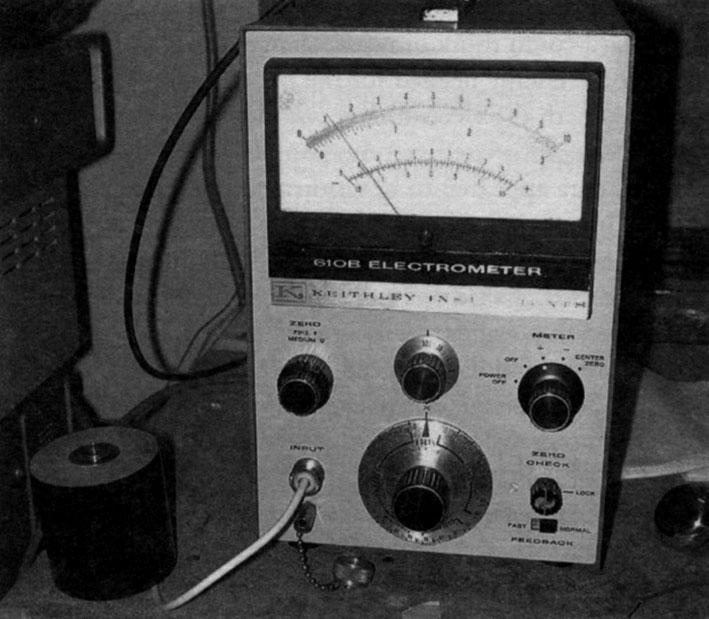
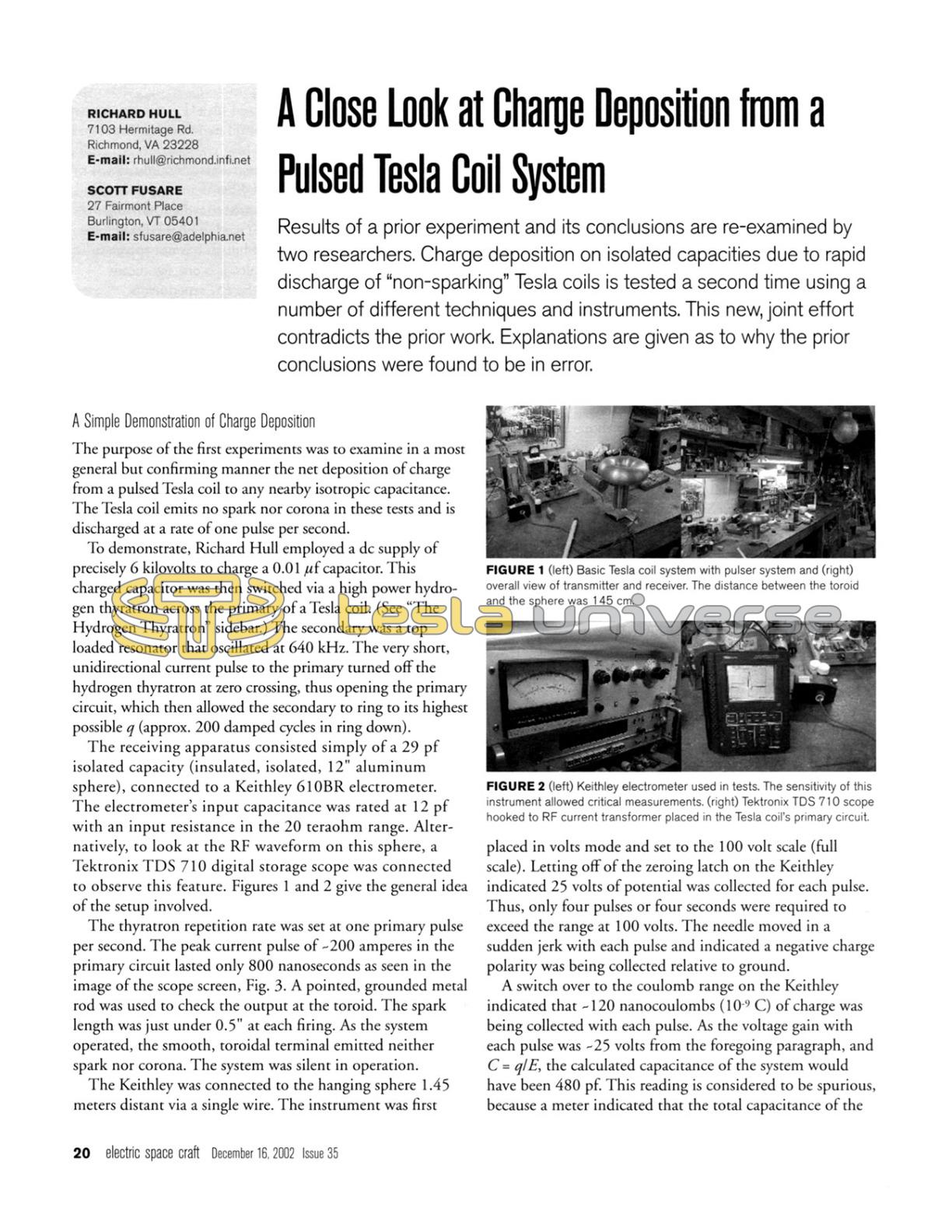
The receiving apparatus consisted simply of a 29 pf isolated capacity (insulated, isolated, 12" aluminum sphere), connected to a Keithley 610BR electrometer. The electrometer's input capacitance was rated at 12 pf with an input resistance in the 20 teraohm range. Alternatively, to look at the RF waveform on this sphere, a Tektronix TDS 710 digital storage scope was connected to observe this feature. Figures 1 and 2 give the general idea of the setup involved.
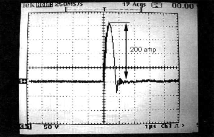
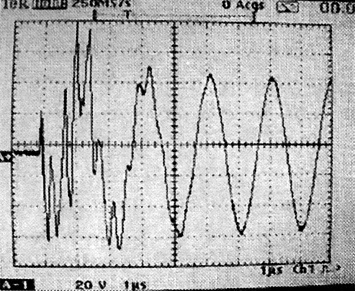
The thyratron repetition rate was set at one primary pulse per second. The peak current pulse of ~200 amperes in the primary circuit lasted only 800 nanoseconds as seen in the image of the scope screen, Fig. 3. A pointed, grounded metal rod was used to check the output at the toroid. The spark length was just under 0.5" at each firing. As the system operated, the smooth, toroidal terminal emitted neither spark nor corona. The system was silent in operation.
The Keithley was connected to the hanging sphere 1.45 meters distant via a single wire. The instrument was first placed in volts mode and set to the 100 volt scale (full scale). Letting off of the zeroing latch on the Keithley indicated 25 volts of potential was collected for each pulse. Thus, only four pulses or four seconds were required to exceed the range at 100 volts. The needle moved in a sudden jerk with each pulse and indicated a negative charge polarity was being collected relative to ground.
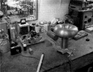
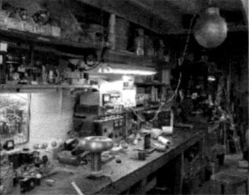
FIGURE 1A. - Basic Tesla coil system with pulser system.
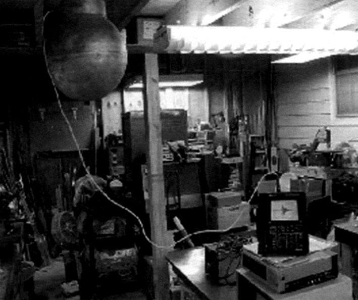
FIGURE 1B. - Overall view of transmitter and receiver. The distance between the toroid and the sphere was 145 cm.
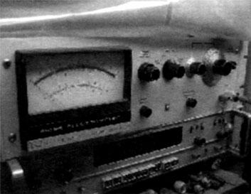
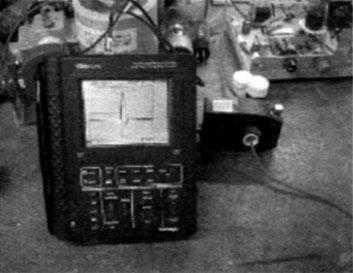
FIGURE 2A. - Keithley electrometer used in tests. The sensitivity of this instrument allowed critical measurements.
FIGURE 2B. - Tektronix TDS 710 scope hooked to RF current transformer placed in the Tesla coil's primary circuit.
A switch over to the coulomb range on the Keithley indicated that ~120 nanocoulombs (10-9 C) of charge was being collected with each pulse. As the voltage gain with each pulse was ~25 volts from the foregoing paragraph, and C = qlE, the calculated capacitance of the system would have been 480 pf. This reading is considered to be spurious, because a meter indicated that the total capacitance of the system was -40 pf. This was double verified via top loading a separate resonator with the large aluminum sphere and its cable and then back figuring from the change in resonant frequency, the total capacitance. This indicated a total capacitance of 29 pf for the terminal and its lead wire. Add to this the shunting of the 12 pf Keithley, and 41 pf is the result. Thus, the coulomb range suffers under the same limitations as the voltage range, being merely an extension of the circuit. Again, all is covered in the Low Level Measurements Handbook by Keithley.
The Hydrogen Thyratron: A Precision, High Energy Switch
Richard Hull, High Energy Amateur Science, Richmond, VA
The hydrogen thyratron vacuum tube was created and designed in three power handling ranges to replace spark gaps for aircraft and, ultimately, ground-based radar. The tube basically consists of a special heater assembly capable of supplying huge numbers of electrons for short periods to support conduction of very high currents at very high voltages through an ionized hydrogen gas atmosphere. The turn-on of this switch can be controlled via a voltage applied to a grid within the tube. This switching action can be precise to within tens of nanoseconds, and support switching rates of up to 2000 pulses per second with peak powers of over 3 megawatts in the largest of the three tubes. One of the key considerations in radar systems, right after high-energy switching, was switching jitter. This was the time, plus or minus, on either side of the point where switching actually occurred. This was very important in radar as this determined ranging data. The hydrogen thyratron filled all the promises of the nearly perfect, maintenance-free switch.
The three classic glass tube hydrogen thyratrons which are often still found at hamfests are the 3C45, the 4C35, and the 5C22, in order of increasing power handling capacity. Such tubes can cost between $2.00 and $30.00 at such events. Most loose, surplus hydrogen thyratrons encountered are either used or pulls from radar units where the jitter in the tube was out of tolerance. As most amateur science investigators' uses are not critically time specific, tubes with terrible jitter, pulse to pulse, are just Tine. All three types of tubes require 6.3-volt filament supplies with increasing amperage in the more powerful tubes. All tubes require a long warm-up period of at least five minutes before being placed into high-power switching situations. All of the tubes have four pin bases of two different types with anode caps on top of the tube. All hydrogen thyratrons run very hot even when not handling power due to the large cathode power requirements.
The amateur experimenter can use the hydrogen thyratron to do some very fast switching in research projects where high dVldt or high dildtpulses are needed. One use is to replace the spark gap in a Tesla coil. Another would be to dump a capacitor's stored energy into a plasma. The only complication is in supplying properly conditioned grid turn-on pulses and shutting off the tube. The grids usually require a 100-volt or greater positive turn-on pulse from a 50Ω impedance source. The pulse must have a rise time of less than 1 us and a duration of at least 1 us. This is relatively easily achieved with modern solid state devices feeding a small pulse transformer. Like all vacuum tube thyratrons and solid state SCRs, the tube, once turned on, will never turn off until either the high-voltage anode potential is removed or its polarity is reversed. This action is normally achieved by using an inductor or coil of wire as the load. The reversal of potential due to normal damped oscillations turns the tube off at the end of the first half cycle. Thus, the classic output is a single, high-power, positive pulse. The pulse duration from a hydrogen thyratron is a function of the natural period of the inductor and any capacitance in the circuit with it.
For more information, refer to G. N. Glasoe and J. V. Lebacqz, Pulse Generators (New York: McGraw-Hill, 1948) and Triton Electron Technology Division Home Page <http:// www.tritonetd.com> 9 August 2002.
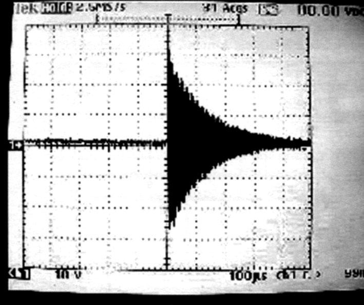
Next, Richard wanted to see the RF waveform received on the large sphere. For this a digital storage scope was connected. The scope, of course, totally loaded the 40 pf capacitor with its 10 megohm input shunting resistance. Thus, no dc component was seen. The waveform and general setup are shown in Figs. 4 and 5.
The resonator frequency of 640 kHz has a period of ~1.5 microseconds. Thus, the 400 microseconds plus ring time shows over 250 oscillations from the totally free ringing secondary. The peak to peak voltage is on the order of 60 volts at this 10 megohm loading.
Figure 3. - Current vs. time trace showing 200 amp, 800 ns pulse. (Current transformer sensitivity was 1 volt/amp.)
Some controls were used to check against other agents at work in the charging. A pointed rod was placed on the toroid of the Tesla coil extending out in midair so that with each pulse, a minor spark or coronal snap into the air was seen and heard. This artifice did not increase nor decrease the earlier recorded data. The same charge was collected with each pulse. Also, the resonator was removed and just the primary was used to send the pulse, but this showed no charge collection at all.
While not the first time Richard had performed this experiment, it indicated with better controls and more quantitative data that net charge was being conveyed from a unipolar pulsed Tesla coil to any and all nearby isolated, isotropic capacitances. The charge appeared always to be negative. The complete mechanism for this was not assumed to be transfer of negative ions or electrons, as no spark or air breakdown was noted. Also, there appeared to be no capacitive coupling of the ac waveform to create a net positive charge, although this might have been possible if some form of rectification was occurring in the receiving circuit.
"...when the ac voltages at the input are large, part of the ac signal may be rectified, causing errors in the indicated dc value being measured."
Low Level Measurements Handbook, p. 3-23
It had been suggested that a simple dissimilar metal junction with minor oxidation might be just the thing to rectify the damped wave. This was a good guess and warranted further study. However, the peak voltages at the teraohm loading level of the Keithley should have been far greater than the 30 volt peak signal of the 10 megohm scope loading. All might have worked out to the 25 volt per pulse noted if this suggested rectifier was of very high forward resistance. Also, the PIV of the single junction rectifier would have had to be very high to avoid flashover and ultimate discharge as the 25 volts added up to higher and higher voltages. Richard planned to extend the range of the Keithley with a custom divider to check out some of the above points.
FIGURE 4. - Secondary ring down of the Tesla coil from single pulse.
Challenges, Refined Experimentation, and Corroboration
Modern, high-efficiency, ultra-fast rectifiers were inserted in the receiver circuit, and the experiment was repeated. The results were puzzling and confusing. The reversals of the rectifiers in some cases changed little, in other cases, dramatic differences were noted. What's more, different rectifiers acted differently in the same connection in some instances. One might have concluded that in some connections, the direction of the inserted diode bucked the assumed rectification in the first experiment. The position of the diode in the receiving setup was also considered in the explanation of some results.
FIGURE 5. - The basic setup for RF waveform viewing.
At this point, Scott Fusare, who had noted possible loop/ grid leak anomalies in a similar Keithley instrument, suggested that the high dVIdt pulses might be playing havoc with the front end of the instrument. According to pages 3-23 of the Low Level Measurements Handbook, 4th ed. (Cleveland: Keithley Instruments, Inc., 1992), "...when the ac voltages at the input are large, part of the ac signal may be rectified, causing errors in the indicated dc value being measured." It was agreed that if the instrument was disconnected and shorted out, it would be out of the equation.
The isotropic sphere would then be allowed to acquire charge in a disconnected state and measured for charge after the source of high dVIdt pulsing was turned off. The instrument could then be reconnected to verify whether the naked sphere was indeed charged as claimed in this experiment. Another benefit, in hindsight, would be the elimination of any possibility of dissimilar junction rectification of the damped RF waveform through the connections to the instrument while charging.
This "definitive" test was performed over several iterations with proper guards and controls in place. Richard set up the coil circuit in his 18°F lab about midnight. He clicked on the 610BR and let it and the hydrogen thyratron filaments warm up for about ten minutes while stomping his feet and watching his breath. It was critical to replicate, exactly, the original experiment.
He found a lot of possible snags and eliminated them. First, he noticed that in order to do the above, he had to ground the spheres lead (to be assured of zero charge), let it hang free, and then hustle just under the sphere, start the pulsing in the coil, let it pulse ten times, then shut off the coil. He then had to whisk his body, again, just inches under the sphere, grab the wire and push it in the banana jack. That left a lot of opportunity for the sphere to image him and his motions. He therefore tried three dry runs with no coil operation. On all three occasions there was virtually no charge collected by passage near the ball.
Richard performed the pulse experiment in volts mode, and the meter pegged instantly on the 100 volt scale negatively, just as if it was connected as in the original experiment. He did this three times, successively. Then, he did the experiment in coulomb mode and in the 10-8 coulomb range. The needle pegged negatively, just as in the original experiment, upon connecting the totally isolated sphere. Again, he did this three times.
He then got the idea that maybe he was now being charged standing near the coil, and passing under the ball might transfer that charge or part of it. Therefore, he did the experiment again in both modes, but this time he walked all around the benchwork 20 feet away to enter from the other side without getting near the ball to reconnect the sphere. Still, full charge and potential were seen.
The waveform in Fig. 6 was taken in an extension of the above experiments and under the same conditions reproduced as faithfully as possible. It shows the first few microseconds of electrical activity recorded on the receiving ball antenna. It must be remembered that it was loaded with 10 megohms due to the scope input impedance, and no dc charge was seen. This is the hidden, compressed first few cycles of the 400 us long damped wave of the earlier waveform. It is suggested that reference be made to the earlier waveform for comparison.
The resonator fill time is generally considered to be that interval before the second zero crossing in some critically coupled systems. This system is not critically coupled, but over-coupled slightly. As the energy flowing in the primary coil was seen to last only ~800 ns, the mysterious activity over the first 3-4 microseconds here would need some explanation. Could this actually be the ball and scope capacitance coupled with the lead-in inductance at the receiver reacting to the initial energy placed on the sphere, and ringing up at its own higher resonant frequency; or is this an actual received signal created back at the transmitter?
Richard could think of no mechanism that might explain the energy needed for the net charging process observed with the electrometer without invoking some form of unappreciated rectification of the RF signal. The original data appeared to be confirmed, thereby exonerating the instrument of possible mischief while being connected during charge collection. Richard could only conclude that charge was transferred, and his original experiment was validated.
But Scott was not convinced.
The Case for a More Commonplace Interpretation
Scott wanted to use a homemade coulomb meter designed around a circuit similar to his Schumann resonance receiver to investigate the propagation speed of the transmission wave, if that was possible. That was going to require a higher bandwidth than professional electrometers offered. Luckily, the solution was simpler than it sounded; the design wouldn't be burdened with all the professional requirements. It also would circumvent the loop stability complication he recently noted on his Keithley 610B. Of course, questions would be raised about the reliability of the homemade instrument, but Scott was prepared to deal with them.
FIGURE 6. - The first few cycles of the damped wave revealed with a magnified time scale.
He repeated the isolated ball experiment in more detail, and his results were still negative. Details of the tests follow:
Figures 7 and 8 show the equipment used. The 6" stainless steel sphere was attached to a 2" PVC coupling with hot melt glue. This in turn rested on a piece of ½" Teflon. A 6' length of silicone insulated HV wire connected to the electrometer. The wire entered through a hole in the benchtop and was held down with a big doorknob cap. The wire insulation touched only the air, with the exception of the ball end and the passage through the benchtop. Everything was carefully cleaned with alcohol. As an insulation check, the sphere was charged via induction and left to set. With about 50 volts on the sphere and a 5-minute wait time, there was no noticeable change. That was good enough for this instrument. The input wire could be removed and held (via the insulation, of course), and then returned, and the readings would still be similar. There was, however, a small change in charge due to the triboelectric effects of touching the wire.
The coil was turned on, giving approximately 1 pulse per second. The electrometer was set in the volts mode. A very repeatable 25-30 volts (negative) per pulse quickly pegged the meter. Then the input wire was removed from the receptacle and hand-held. The Tesla coil was allowed to pulse 20 times, several times more than was needed to peg the meter. The wire was plugged back in. At best, very small voltages, <5 volts, were recorded. These small voltages corresponded to the triboelectric charging seen in the first experiment. No significant reading was observed.
Next, the 610 was set to read coulombs. On the 10-10 range, a single pulse gave a half- to a full-scale reading (negative), implying there were around 100 picocoulombs per pulse. Still on the coulombs setting, the meter was adjusted to the 10-9 range. A pulse reading of one minor gradation was recorded, implying there were approximately 10 picocoulombs per pulse, an order of magnitude less. Still on the coulombs setting, the meter was then adjusted to the 10-8 range. Hundreds of pulses were allowed to occur. No charge was recorded - none! According to the results from the 10-10 range, more than enough charge should have accumulated to peg the meter on this scale.
All changes in charge appeared to result from the loop issue mentioned earlier. The coulomb range results were the clincher, as the loop effect has a threshold voltage that must be exceeded before it occurs. The increase in integrating capacitance, which corresponds to the increases in coulomb range, also forms a larger voltage divider holding down the voltage on the ball. Eventually, in the 10-8 range experiments, the voltage fell below the threshold.
More Evidence
After discussing the experimental results with Richard, Scott performed a few more experiments. First, the 610B electrometer was replaced by a 602 (solid state front end), and the same setup and spacing were used as in the previous work.
Measuring voltage, this instrument had a maximum reading of 10 V, so given the 25-30 volts per pulse seen on the 610B each pulse should have pegged the meter. Instead, each pulse registered approximately 1 volt (negative). Occasionally, an increase of 5 volts or more was observed, but that was rare. Running the isolated ball test, the results were the same as with the 610B: The only changes observed were attributable to triboelectric charging from touching the silicone insulation of the connecting wire.
Measuring charge with the coulombs scale on the 10-10 range, 10 picocoulombs (negative) of accumulated charge per pulse registered. On the 10-9 range, nothing registered.
Next, Scott substituted an aluminum collector for the stainless steel ball. The new collector was a 14" spun aluminum Van de Graaff terminal. Using the 610B, the results were unchanged, save a slightly larger per pulse increase on the volts-per-pulse scale, about 40-50 volts. So, the 610B and the 602 did not give the same results; there was an order of magnitude difference. The aluminum collector did not show a charge accumulation, and the per-pulse voltmeter reading did not increase proportionally to the surface area. This further supported the assumption that the apparent charge transfer was merely an artifact of the instrumentation.
The Lindemann Electrometer
The Lindemann electrometer might well be considered to be the pinnacle of refinement in mechanical electrometers. Capable of detecting current flow in the 10-14 ampere range, it is virtually as sensitive as many modern electronic electrometers. The Lindemann is a member of a large family of instruments called quadrant electrometers designed in the early twentieth century for quantitative work in radiation measurement and sensitive photometry. The electrometer used in these experiments was a very small version designed for astronomical photometry.
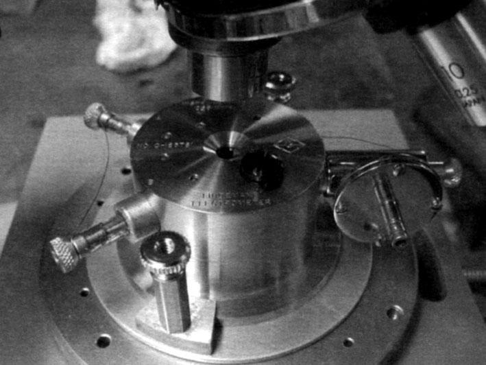
This particular electrometer suspends a 5-micron wire on a 3-micron quartz fiber. The tiny wire is suspended between four quadrants of isolated metal. The case of the Lindemann is always metallic and acts as a shield against stray pickup. Each diagonal quadrant pair is connected electrically. As a charge appears on the wire, it is torqued against the fiber to deflect between quadrants. The amount of deflection is an indication of the charge applied. The wire's deflection is read against a scale. This scale is contained in an eyepiece of an external optical telescope focused on the fiber through a viewing hole or window on the electrometer. All Lindemann electrometers have a variable bias voltage applied to allow zeroing of the wire's image against the scale and to establish a known field within the device. This optimum field voltage is predetermined by the manufacturer and written on a label inside of the wooden storage case for the instrument. The unknown input signal shows up on the suspended wire and deflects it via coulombic attraction/repulsion until it reaches a like-field equilibrium within the established field.
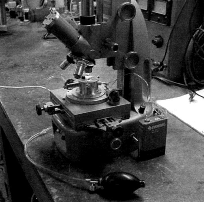
Figures 9 and 10 are a couple of images of the Lindemann hookup, figure 9 shows the entire setup. The squeeze bulb is used to shunt the input to ground for resetting just like on a Keithley. The 45-volt B battery is for biasing the quadrants, and the potentiometer on the stage is for balancing and centering the quartz indicating fiber. The hookup used is common to all quadrant electrometers and is shown schematically in John Strong, Procedures in Experimental Physics (Bradley IL: Lindsay Publications, 1986; reprint, Englewood Cliffs, NJ: Prentice-Hall, 1938), p. 233, Fig. 10, Circuit C. The Lindemann is explained in some detail on page 243.
- Richard Hull
FIGURE 9. - Lindemann electrometer setup.
FIGURE 10. - Closeup of electrometer.
While working with the 610B after the coil was off, Scott allowed his cotton shirt to lightly brush the floppy, silicone-insulated lead he and Richard referred to as the noodle wire, something he took care to avoid in the previous tests. This pegged the meter negative on the 100 volt scale. He asked Richard if something similar was the cause of the accumulated charge observed during the isolated ball tests.
Isolating the Instrumentation from the Experiment
Richard verified Scott's triboelectric charging of the noodle wire with the slightest brush. He then investigated the effects of measuring charge with a coulombic Lindemann electrometer, rather than a complex electrometer with unknown, built-in electronic side effects. (See "The Lindemann Electrometer" sidebar.)
As noted before, this electrometer is extremely sensitive and in every way the equal of the Keithley, but it is a lot more bother to use. The experimenter must hover over the instrument and constantly rezero it, due to ceaseless static pickup; and he experiences eyestrain as he peers into a microscope ocular to obtain data. Now, in hindsight, the bothers are worth it. The $6000 Keithley electrometer was indicating a continuous charge collection occurring on a large isolated sphere while operating a nearby Tesla coil, but the Lindemann indicated no charge buildup. It turned out that the method of construction of the feedback loop within the Keithley could not handle signals of large amplitude which oscillated at a frequency much above 500 Hz. In other words, its own internal circuitry generated the error.
Such false indication possibilities of the electronic electrometer are well-documented in the Keithley Low Level Measurements Handbook. (See, for example, "Electrostatic and Electromagnetic Issues," pp. 3-70.) It must be stated that this is no fault of Keithley or the instrumentation, but more a naturally arising characteristic of the electronics needed to construct the sensitive input section of the instrument. The signals were of too high a potential, too fast a rise time and often too rapid a repetition rate for the instrument to follow without introducing artifacts. The Lindemann, on the other hand, relied totally on coulombic action affecting a mass in an unmistakable and well-understood manner. There were no hidden electronic, looping/feedback artifacts, just real masses reacting to real forces in an electrostatic manner.
The bad news is, the magic is gone. The good news is, hopefully we have learned something, and armed with items like the Lindemann, we will not be fooled again.
Mea Culpa
It is in the spirit of good science that I must now publish a formal retraction of the interpretation of a result obtained over the last four years, regarding the electrostatic charging of remote, isolated isotropic capacitances with a Tesla coil. It appears, in the light of new work and the discovery of a well-disguised problem associated with the professional electrometers used to take data in the past, that no net charge is placed on remote conductors by a functioning Tesla coil.
In recent months, I was involved with new experiments using the short pulsed hydrogen thyratron triggered Tesla coil. Again, results were showing the net charging effect reported all along. I started corresponding with my friend and fellow researcher Scott Fusare on a related matter involving Schumann resonances. He had assembled a nice homemade electrometer of high bandwidth and was getting some nice results. Scott had wanted to test out some of the electrostatic experiments reported in ESJ. Armed with a similar electrometer to my own (Keithley 600 series), he began his effort and reported that the Keithley might have a problem reporting correctly on fast, high dVldt pulsed signals over 1 kHz.
It turns out he was correct. After several days of intense cross experimenting, emails, and phone calls, it was determined that I should use the ancient, but fully coulombic, Lindemann electrometer I had as an antique curio, to verify, once and for all, no charge collection. The venerable old instrument was a bear to stabilize and zero, but the effort was repaid in the absolute and irrevocable conclusion that the remote isotropic capacity was not charging during Tesla coil operation.
The lesson to be learned is to never trust an instrument completely. Try and find methods to use other instruments to cross check your results.
I wish to thank Scott Fusare for sharing directly in this effort and apologize for the errors and perhaps misdirection of others' efforts. I look forward to working as a team on future efforts where it is readily seen that two or more heads are often better than one.
- Richard Hull
Downloads
Downloads for this article are available to members. Log in or join today to access all content.
Downloads
Downloads for this article are available to members. Log in or join today to access all content.