Nikola Tesla: Colorado Springs Notes, 1899-1900 Appendix II

The classical Tesla transformer with adjusted primary circuit and self-oscillating secondary coil, particularly when so fitted to achieve the highest possible secondary voltage with minimal capacitance load, cannot be exactly calculated on the basis of theory of circuits with concentrated parameters. Resonant frequency of a free secondary greatly depends on the position of that coil relative to the objects surrounding it (particularly metal ones) so that calculation of inductance and capacitance of the coil based on quasi-static analysis is not particularly successful. As of late a new approach was developed for the calculation of the secondary circuit based on the theory of helicoidal transmission line with a slow electromagnetic wave. In this case current wave is considered traveling along the coil at a speed close to light speed in free space and electromagnetic wave traveling along the axis of helicoid at a considerably lower speed.

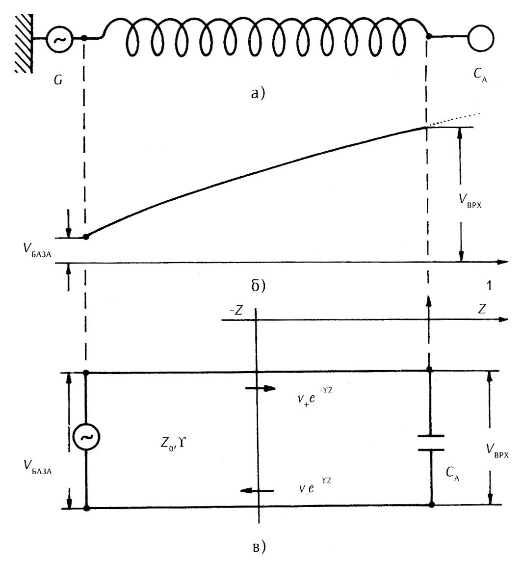
Voltage at a cross section of excited helicoidal line (cf. figure 3P) is a sum of direct and reflected wave of voltage, which is analytically expressed by the known relation:

V(z) = V₊e^-yz + V_-e^+yz

Where γ = α + jβ, complex coefficient of propagation along helicoid. A component of direct wave at the line end is V₊, while component of reflected wave is V_-. Distance is measured from the line end. The complex coefficient of reflection at the line end is a relation of reflected and direct voltage at the line end and expressed depending on the closing impedance Z_L and characteristic impedance Z_O via relation:

Γ₂ = $! {V_{-} \over V_{+}} $! = $! {{Z_{L} + Z_{O}} \over {Z_{L} - Z_{O}}} $! = |Γ₂|e^jφ2

On the excited side of the line, the complex coefficient of reflection is a relation between direct and reflected voltage at the beginning of the line:

Γ₁ = $! {{V_{-}e^{-yl}} \over {V_{+}e^{+yl}}} $! = |Γ₂|e^-2αlφ₂ - 2βl

The degree of standing waves at the line end is found from the relation:

S₂ = $! {{|V_{+}|+|V_{-}|} \over {|V_{+}|-|V_{-}|}} $! = $! {{1+|Γ_{2}|} \over {1-|Γ_{2}|}} $!

On the conductor without losses the degree of standing waves is not changing along the line and remains the same as at the beginning of the line. On the line with losses it depends on the input impedance and characteristic impedance, namely on the module of the coefficient of reflection at the line input:

S₁ = $! {{1+|Γ_{1}|} \over {1-|Γ_{1}|}} $! = $! {\tanh\left[{αl + \tanh^{-1}\left(1 \over S_{2}\right)}\right]} $!

for standing waves greater than 6, the preceding equation can be simplified:

1/S₁ = 1/S₂ + αl

with an error less than 1%. In case when the end of line is capacitance loaded and without loss S₂ →∞, so that S₁ = 1/αl.

To obtain maximum voltage at the open end of the secondary, the parameters of a helicoidal line are chosen so that it behaves at the working frequency as a quarter-wave line. If at the input of the line of l length the input voltage is then the voltage at the end line is expressed by relation:

V_basis = V₊[e^{(α + jβ)l}₊Γ₂e^{-(α + jβ)l}]

length of the input voltage is then the voltage at the end line expressed by relation:

V_top = V₊(l + Γ2).

By eliminating V₊ from the two preceding equations the ratio of excited voltage and voltage at the end of line is obtained.

V_top/V_basis = $! {{1 + Γ_{2}} \over {e^{(α + jβ)l} + Γ_{2}e^{-(α + jβ)l}}} $!

To obtain maximum voltage at the line, output it is necessary that the nominator of the above equation at the right side be the least possible. For further calculations, the coefficient of weakening and phase coefficient of helicoidal line are expressed in parameters of the units of length of lines: resistance, conductance, capacitance and inductance (r, g, l, c). In cases when weakening is not great, as can be considered in the observed case, the coefficient of weakening is found from the relation:

α = $! {r \over 2Z_{0}} $! + $! {gZ_{0} \over 2} $! ≈ $! {r \over 2Z_{0}} $!

because, usually conductance per unit of length is significantly lower than resistance per unit of length of the conductor. For the calculation of voltage at the end and beginning of the line it is necessary to know αl, namely rl, which in the case considered represents total resistance of conductor of helicoidal line. Phase coefficient depends on the factors of reduction of phase velocity of propagation of the phase of the wave along the axis of helicoid V_f and is calculated from the relation:

β = $! {2 \pi \over λ_{g}} $! = $! {2 \pi \over V_{f} λ_{0}} $!

To calculate coupling with other elements of the transformer it is necessary to know input impedance of the helicoidal transmission line and it is calculated based on the relation:

Z_ul = Z₀$! {{1 + Γ_{2}e^{-2yl}} \over {1 - Γ_{2}e^{-2yl}}} $! = Z₀$! {{1 + Γ_{1}} \over {1 - Γ_{1}}} $!

For practical application of the above theory it is necessary to connect physical parameters of Tesla's transformer and parameters figuring in theoretical formulae. A physical helicoidal line is characterized by the diameter of the coil, thickness of wire, distance between conductors, length of turns and material from which the wire was made. On the basis of the mentioned data, the following is determined:

Factor of reduction of phase velocity V_f which figures in the term for the phase coefficient

V_f = $! {V \over C} $! = $! {\left[{1 + 20\left({D \over S}\right)^{5/2}\left({D \over λ_{0}}\right)^{1/2}}\right]^{-1/2}} $!

where λ₀ is wave length in free space, D is diameter of helicoid, S is the distance between two neighboring turns. All the values should have the same dimensions.

Weakening of helicoidal transmission line is calculated from the relation (for copper conductors):

al = $! {{198,44\left({H \over D}\right)^{1/5}} \over {d_{mm}Z_{0} \sqrt{f_{MHz}}}} $!

where d_mm is diameter of wire in millimeters, f_MHz is frequency in mega Hertz, H is the length of the coil in the same unit as D. The third parameter is effective characteristic impedance:

Z₀ = $! {{60 \over V_{f}} \left[{ln\left({4H \over D}\right) - 1}\right]} $!

With the above theory it is possible to calculate two types of Tesla's transformers. One is the classical type with resonant primary of small inductance and the secondary in the shape of long coil that is calculated as a helicoidal line. The primary circuit excites helicoidal line and at the end of the line maximum voltage is achieved when electric length of helicoidal line is λ_g/4. If closing capacitance is located at the end of the line then the line must be shortened to achieve the maximum voltage.

Another type of high voltage transformer, developed by Tesla in Colorado Springs, has three coils: primary and secondary coils are in a relatively strong inductive coupling and the third, extra coil is not practically inductively coupled with the first two. We may consider that the third coil practically behaves as a helicoidal line that achieves a high degree of multiplication of voltage if properly dimensioned and charged from a source of low impedance. Such a coil was connected by Tesla to the secondary of the transformer of high diameter (see, for instance, data about transformer, provided in his Notes on October 2, 1899) and achieved voltages of the magnitude of 10 million volts. In doing so, he started from the voltage of the magnitude of 20 kv/133 Hz and achieved the increase of voltage by some 45 times. The increase in voltage of that magnitude in the domain of high frequency currents with which Tesla worked is not at all simple. In this case a simple Tesla transformer with two coupled oscillating coils requires ratio of capacitance of the primary and secondary of some 2,000. For such a ratio and capacitance of the secondary of 200 pF the primary capacitance should be above 0.4 microfarad, which is at least three times bigger than that which was sufficient for Tesla.

Tesla's theory of an additional coil was ultimately simple. He calculated (and then measured at 133 Hz) inductance of the additional coil starting from a simple formula of inductance of an endlessly long coil and connected it to the free end of the coil of the antenna pole so obtaining the third oscillating circuit in a weak inductance coupling with the other two coupled circuits. He experimentally established that considerably higher voltage is achieved than with only two coupled circuits, namely considerably stronger antenna current. He made no attempt at more complex analytical calculations, since experimental perfection for him was a pathfinder and inspiration for new variations. When the operation of Tesla's transformer with sparker is studied today, computer technique may be resorted to in scaling variations and after considerable trouble arrived at a series of replies that Tesla obtained with his simple theory and capability of experimenting and extraordinary successfully interpreting and applying of the results on his further investigations.

The operation of Tesla's transformer with two oscillating circuits excited by sparks is possible to describe by an analytical model based on the above described Oberbeck's model, but at considerable widening thanks to the computer.

75