Atmospheric Fields, Tesla's Receivers and Regenerative Detectors

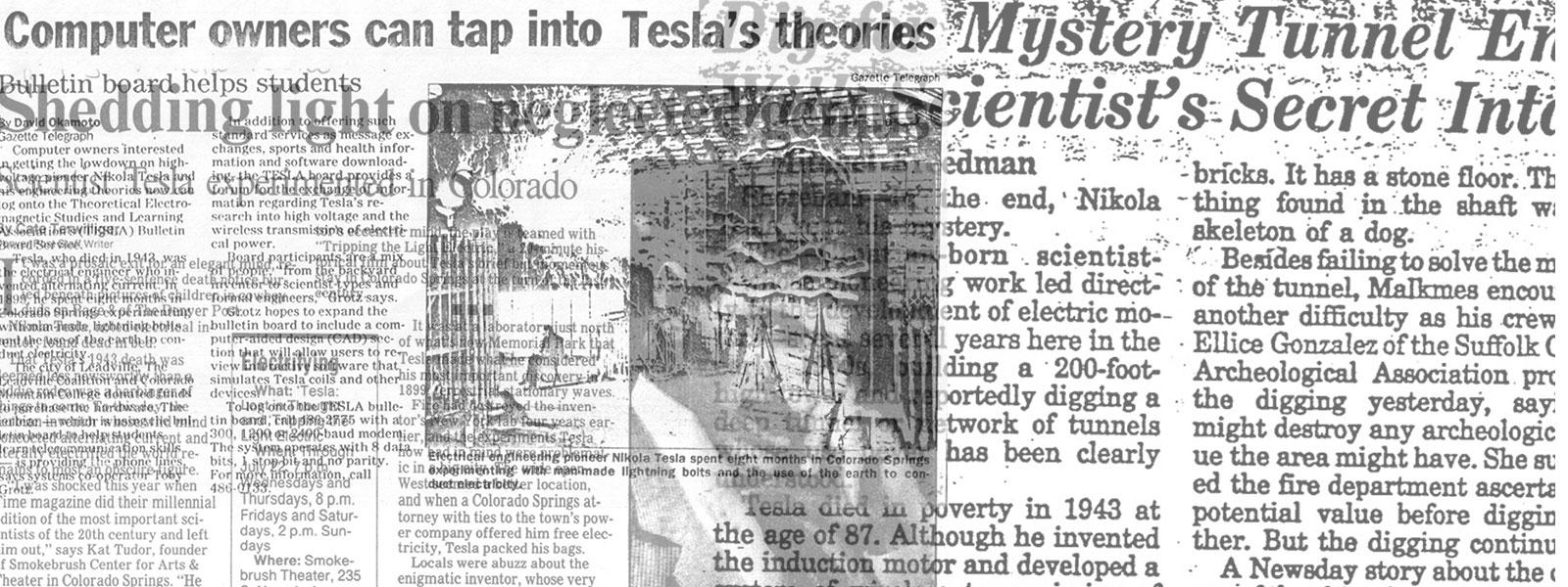
This paper reviews our experimental and analytical research into the sensitive detector circuits employed by Nikola Tesla during his famous lightning observation experiments in Colorado. Using Tesla’s laboratory notes, correspondence, and patent applications, we have reconstructed models of his apparatus which reveal an unanticipated level of sophistication. His 1899 coherer circuits not only include distributed high Q helical resonators, but also RF feedback, a primitive form of heterodyne (mixing), and regeneration techniques. The phenomenology is correlated to the RF work of Mahlon Loomis, Edwin Armstrong and others.

While experimenting in Colorado ... I had perfected a wireless receiver of extraordinary sensitiveness, far beyond anything known.-- Nikola Tesla (Albany Telegram, Feb 25,1923)

The free oscillations which are set up during the periods of negative resistance are directly proportional to the amplitude of the impressed EMF.... amplification of 400,000 can be obtained: -- Edwin H. Armstrong (Proceedings of the IRE, 1922, p. 244)

Introduction

We have pursued the published literature of Nikola Tesla for several decades, now. While we must confess that on any given topic our initial attitude was usually one of incredulity with this brilliant scientist, yet we have, over the years, found by experimental investigation that Dr. Tesla’s technical assertions and comments have been reliable and trustworthy. (If he said he saw something or did something in the laboratory, then he saw it or did it. And, you can take it to the bank.)

This was true concerning his ‘Extra Coil’ resonator. What was lacking when we started on that apparatus was a modern critical engineering study - both experimental and analytical. It was true concerning his laboratory production of ‘Ball Lightning’. What was again lacking was an engineering understanding of the fireball generation apparatus. When this was obtained by an interactive research program, the experimental and analytical verification followed in a matter of hours.

Let us make it transparently clear that the engineering analysis did not come about by mere ‘pencil and paper’ contemplation. Years of failure - in both theory and experiment - were required to finally hammer out the (now) obvious. [Those academicians and journalists among us reading this haven’t a clue as to what we just said! ... Not a clue!!]

Engineering is not a cerebral exercise. It’s not mathematics. And, it’s certainly not computer simulation. Although, if their limitations are understood, these are great instruments for lessening the toil and clarifying the understanding of the engineer and inventor. The problem is theological: while analytical and numerical models may be explored, optimized and exploited, they’re confined in an isolated box that is no better than their human architects. In the real world of nature we are bound only by the fundamental limits of creation.

We have puzzled over Tesla’s receivers, both those used in New York and those used at Colorado Springs, and we would like to share our investigation of the latter. At Colorado Springs Tesla employed a remarkable variation of the popular “coherer”. Interestingly, the coherer fell into disuse as a detector around 1906, and its physics of operation was never really understood. The ignorance remains to this day.

We think that an understanding of Tesla’s ‘sensitive device’ will throw considerable light on how he arrived at certain experimental conclusions. We want to discuss both his version of the coherer and its employment in several of his remarkable receiver configurations, especially those with feedback. Yes, this brilliant man of science was employing negative resistance and nonlinear feedback to his advantage prior to the turn of the century! But first, let us review some background history to get things into perspective.

Part I. Coherer History

1. Munck

Historically, the origin of the coherer can be traced to Benjamin Franklin’s experiments with a cylindrical glass tube, filled with earth and having electrodes in both ends, as described in 1748.

About ten years later Edward Delaval (1729-1814) used the same configuration to create the first (more-or-less linear) ‘resister’ (his spelling) using various powders in the tube.[1] Following on Franklin’s electrostatic discharges and Delaval’s resistors, Swedish physicist P.S. Munck of Rosenschold (1804-1860), in his experiments of the 1830’s, noted that,

“...when the Leyden jar had been charged to a sufficiently high voltage, discharge drastically lowered the powder resistance, which then remained low as long as the powder was not poured out of the tube. When the tube was refilled with the same powder, the resistance became high again and shaking the tube also restored the initially high resistance value.”[2,3]

A device based on this principle was patented in 1866 by the Varley brothers of England as a lightning protection device for land-line telegraph (a forerunner of the Varistor). When the induced voltage on the wires exceeded a certain value, the device conducted and protected the telegraph operators from static discharge.

Tesla acknowledged this device in his own US Patent #613,809:

“Another such contrivance, less sensitive but more readily available, which has been since long ago known and used as a lightning arrester, in connection with telephone switchboards for operating annunciators and like devices comprises a battery the poles of which are connected to two conducting terminals separated by a minute thickness of dielectric. The electromotive force of the battery should be such as to strain the thin dielectric layer very nearly to the point of breaking down, in order to increase the sensitiveness. When an electrical disturbance reaches a circuit so arranged and adjusted, additional strain is put upon the insulating film which gives way and allows the passage of a current, which can be utilized to operate any form of circuit controlling apparatus.”

2. Branly

Edouard Branly (1844-1940) discovered in 1890 that the device did not actually have to be physically connected to a source.(‘) A nearby spark discharge (not only from electrostatic sources but also from high voltage induction coils) lowered the electrical resistance of the powders dramatically (from megohms to ohms). To Branly goes the credit for discovering the go/no-go AC field detector mode of coherer operation.

In US Patent #613,809, Tesla notes:.

“Again, another contrivance capable of being utilized in detecting feeble electrical effects, consists of two conducting plates or terminals which have preferably wires of some length attached to them are bridged by a mass of minute particles or other conducting material. Normally, these particles, lying loose, do not connect the metal plates, but under the influence of an electrical disturbance produced at a distance, evidently owing to electrostatic attraction, they are pressed firmly against each other, thus establishing a good electrical connection between the two terminals. This change of state may be made use of in a number of ways for the above purpose.”

3. Lodge

While conducting experiments with a “Branly tube” in 1890, Sir Oliver Lodge (1851-1940), who had performed spark gap RF detection experiments as early as 1889, discovered its remarkable sensitivity to RF oscillations. [5,6] Lodge found that when RF oscillations were impressed upon metal filings and powders, the resistance fell from extremely high values to very low values the same as with static discharges. Furthermore, placing a battery in series with the RF triggered coherer permitted a DC current to flow with sufficient strength to close a relay and drive a Morse inker or ring a bell (an RF controlled DC switch).

He also found that the original resistance was restored to its high

value by mechanically tapping the device. (See Figure 1.) Furthermore, he determined a secondary mode of operation of the coherer in which it functions much like a diode envelope detector of today. In this mode the nonlinear resistance of the medium is exploited to give RF rectification. (See Figure 2.)

Branly did not like the term ‘coherer’ and he refused to use the expression. In fact, on December 6, 1897, in an objection to Lodge’s introduction of the nomenclature, Branly wrote,

“This expression is based on an incomplete investigation of the phenomenon and on an inexact interpretation; I have proposed the name radio conductors, which recalls the essential property of discontinuous conductors to be excited by electric radiation.”

{Susskind has declared that this is very likely the very first use of the term radio in a communications context.[7]}

Note that so far, there are two conventional modes of operation for the coherer:

1. the RF controlled “go/no-go” switch [which requires repetitive de-cohering], and
2. the nonlinear resistance (diode) mode of operation [which requires extreme mechanical stability].

Extreme is an appropriate word, too. Vivian Phillips, in his book Early Radio Wave Detectors, Peter Perrgrinus Press, 1980, quotes A.H. Taylor’s 1903 remarks that to get his coherer to operate in the envelope detector mode he had to perform experiments late at night, when no electric cars were running, the campus had to be quiet, he had to turn off the clocks, stop the thumping in the steam pipes, etc. The slightest mechanical jar would “abruptly terminate” the envelope detector mode of operation (pg. 29). Our experience full concurs with his observations!

Phillips goes on to quote W.H. Eccles who defended the coherer by saying in 1907,

“The coherer’s reputation for erratic behavior is wholly due to the performance of samples made in a slipshod manner. Coherers so made might aptly be compared with homemade false teeth.” (pg. 60).

4. The Great Coherer Debate

As mentioned above a substantial debate arose over the actual physical operation of the coherer. In a 1992 review article Kryzhanovskii wrote,

“Lodge coined the term coherer from the Latin cohaerere (to stick together), keeping in mind the sticking of the filings to each other under the action of electromagnetic waves. Branley did not use the term “coherer”, which received extensive circulation, because he disagreed with the conductance mechanism which Lodge suggested. Branley called his device a radio conductor. The fact that the device becomes a conductor by the action of electromagnetic radiation is emphasized by this term. The controversial physical mechanism, which has not been completely determined even now, did not delay the practical use of the coherer.”[8]

Despite the existence an extensive literature on the topic of coherers [9, 10] (see almost any early book on wireless), their physics is surprisingly obscure! [11] The best discussion that we have seen was presented by Gindin and Vol’pyan, who trace the three views concerning the nature of coherers advanced in the 1890’s:

“Lodge[12,13,14] believed that the reason for the increase of the conductivity of the powder under the action of the field is the formation of a current-conducting path (bridge) due to the aggregation of particles under the influence of electrostatic forces; these forces ‘strip’ insulating films from the surface of the particles, in particular oxide films.

According to Auerbach, [15] the role of the field is purely mechanical. The field induces a relative disposition of the particles such that it ensures a higher conductivity of the powder.

By virtue of surface forces, the resulting structures are maintained also after the removal of the field.

Branley [16,17,18,19] believed that the layers of insulating dispersion medium between the powder particles are ‘modified’ on application of the field and become conducting.”[20]

Apparently, extensive experimentation (and microscopic optical observation) led to the popular conclusion that Lodge’s explanation, in terms of the formation of conducting bridges in the coherer powders, was the correct one. Fractal-like microscopic bridges and filaments are actually observed in the coherer powders. However, to the present date the actual electrical behavior and physical processes involved are not commonly understood. Kryihanovskii has even suggested that the physical operation of the coherer is quantum mechanical, and that Branly’s device foreshadows quantum theory.

“The insulating layer which separates the conducting particles, becomes conducting under the temporary action of high frequency currents; and [quoting Branly] ‘The conductor particles do not necessarily have to touch each other in order to conduct an electric current. In this case, the insulation serves mainly to maintain a definite gap between particles.’ Thus, Branly predicted the tunneling effect thirty-three years before the founding of quantum mechanics.”[21]

In spite of the fact that the physics of coherers was (and still is) understood poorly, remarkable strides were made in wireless by their use between 1890-1906.

We should probably also mention the carbon microphone detector of David Hughes (1831-1900) [who’s work in the US, though not publicly released until 1899, was contemporaneous with Mahlon Loomis, and predates Hertz’s by a decade], and the impressive investigations of Popov (1859-1906), Sir Jagadis Chunder Bose (1858-1937) [who systematically examined materials for coherers, believing that the operation depended upon a molecular stress-strain relationship], and Marconi’s mentor, Augusto Righi (1850-1920). However, let us move directly to Marconi’s use of the coherer.

5. Marconi

The talent of Marconi (1874-1937) seems to have been his ability to assimilate the work of others into promotable systems. Remarkably, even at this late date and in spite of the overpowering evidence to the contrary, there are still those that continue to allege the persistent myth of Marconi’s priority in the invention of radio. The historical technical evidence just does not support this delusion.

The 1909 Prize was shared with Ferdinand Braun (1850-1918), Director of the Physical Institute at Strasbourg, who was cited for his development of wireless. Braun is shown in the photograph of the 1915 IRE banquet (along with Stone, Zenneck, Lowenstein and Tesla) in the front of Anderson’s 1992 book, Tesla on His Work with AC.

In Figure 3 we show Marconi’s 1909 Nobel Prize’ sketch of his first system of wireless telegraphy and a subsequent development. The broadband detector is untuned. (At one time of the sketch Marconi thought that having a large antenna capacity was the secret to wireless. Later he decided that it was the length of wire in the antenna.) The reader should note the RF circuit, the superposed DC control current path for the battery and relay, and the isolated DC path for the battery driven Morse indicator.

Next, in Figure 4 we show Marconi’s Nobel Lecture sketch of the receiver which he used on Signal Hill in Newfoundland. Note again the injection of RF to the coherer through the “jigger” (the coupled coils), and the DC path to drive the relay (an RF bypass capacitor at the top keeps the RF out of the external DC path). The relay drives an external Morse indicator.

Where are the famous’ earphones? Recall that Marconi, using his coherer, would not have heard the Morse letter “s” (dididit), but rather the coherer response corresponding to the letter “s”, which would have been a stream of clicks between thumps of the decohering tapper.

Marconi’s term “jigger” is obscure in origin. It may have arisen from the picturesque idea that the antenna primary circuit “pours” some of the RF into the secondary circuit, like the measure used in mixing drinks, and thus hark back to his relatives in Ireland. Or it may be related to the aftermost mast in the stern of a ship.

Marconi has said that his earliest experiments were in 1895 using a Branly coherer on his father’s estate in Italy. Unable to stimulate interest in Italy, he went to London and filed for his first wireless patent in 1897, and subsequently linked England and France by wireless in 1899. Marconi’s North Atlantic coherer reception occurred between 1500-1900 GMT on Thursday, December 12, 1901. The 25 kw spark transmitting station at Poldhu, England had been designed and constructed by J.A. Fleming and RN. Vyvyan.

6. Slaby

When Adolph Slaby was permitted to examine Marconi’s early coherer receiver of 1897, he and Count George von Arco were able to see an inherent weakness in the disposition of the elements.

Slaby was able to increase the sensitivity of Marconi’s detector by more than an order of magnitude by simply using the voltage rise due to VSWR [Where have we seen that before? Starting in 1892, who taught this all over Europe and North America, and subsequently patented idea on two continents?]

Aitken discusses the weakness of Marconi’s version:

“In his original circuit the coherer was connected directly between the antenna and ground.

The coherer was a voltage-actuated device. It responded to differences in potential between its terminals. Placed directly between the base of a vertical antenna and ground it was at a point where the voltage differences were minimal, for the distribution of charges in a vertical radiator is such that the currents are maximum and voltages minimum at its base, while the reverse is true at its tip.

The coherer, in other words, was in precisely the wrong place. Small wonder that the coherer was an insensitive detector. [22]

Additionally, the Telefunken, or Slaby-Arco, system makes use of the fact that the V_max occurs at the appropriate positions only at the desired frequency, and thus provides a certain degree of selectivity and interference suppression. (See Figure 5.) Many years later, Dr. W.A.H. von Arco, of Telefunken in Berlin, would write to Tesla (“dem geniallen Altmeister der Radiotechnik”) and state,

“When I entered the world of high frequency as Slaby’s assistant in 1897, the 1895 German translation of Tesla’s Works gave Slaby and I our essential foundation for high frequency techniques.” [23]

Telefunken built its business on the patents of Slaby, Arco, and Braun with state support.

7. Tesla

Our main interest in the coherer arises from Tesla’s use and remarkable improvements of the device during his 1899 Colorado Springs experiments. The coherer and Tesla’s various receiver configurations occupy a substantial amount of his efforts at Colorado Springs. The thought has occurred to many that if one is to ever understand how Tesla arrived at various numerical data and physical conclusions, then one must understand the operation and limitations of his receivers. From his published Lectures, it is clear that initially Tesla used gas filled lamps, and tuned circuits with small incandescent lamps (a wave meter circuit) to demonstrate RF in the early 1890s.

We are introduced to a surprisingly extensive use of magnetic detectors (which hark back to Mahlon Loomis’ [24] work in the 1860s-1880s) in the mid 1890s in Lee Anderson’s book on Tesla’s work with AC. This was a decade before Marconi [25], Fessenden, De Forest, [26,27] Shoemaker, and others began to patent their magnetic detectors. Interestingly, Marconi rejects the coherer and turns to magnetic detectors in May, 1902 (as do de Forest, Shoemaker, and others).

(Strangely, all of the latter bear a striking resemblance to those shown in the notebooks of Mahlon Loomis in the 1860s and 1870s!) [28,29] Tesla had transmitted and received more than 30 miles, prior to 1897, with this technology. [30]

Both the Colorado Springs notes and the legal briefing Tesla gave to his attorney in 1916 show that he used magnetic detectors. Tesla made many variations of the magnetic detector and found them to be very useful as a low impedance (current driven) detector. However, with his high voltage resonators, he needed a high impedance (voltage driven) detector. These conditions were very favorable for the employment of the coherer (as was noted in the Slaby-Arco scheme above).

Furthermore, in Tesla’s 1899 Colorado Springs Notes (and in the contemporaneously filed patent applications) what we see, almost exclusively, is an innovative development of sensitive receivers that utilize coherers in a detector stage employing locally generated RF injection and a third mode of coherer operation. We will return to this below.

Part II. Electrical Characteristics of the Coherer

1. Early Operation of Coherers

The early use of the coherer was that of an RF “detector”, not in the sense of how we use “demodulators” today, but rather for determining whether RF was present or not present. The original employment did not even use a tuned circuit ahead of the device but, as an E-field detector, merely connected it directly to a short piece of wire.

Later, earphones were placed in series with the coherer and capacitance shunted for RF bypass. The presence of RF would cause a click in the earphones, and then no more clicks would be heard until the coherer was tapped or shaken. The same circuit was also used with a galvanometer in place of the earphones. (Realize that this was not an analog field strength meter because of the one-shot nature of the coherer.) To enhance the operation of the meter, a small battery was placed in series with the galvanometer and an RF choke, and these three elements were shunted across the coherer. The coherer still had to be shaken to allow it to detect RF once again.

There were many ingenious methods developed to shake or decohere the metal filings. Decohering was especially a problem in the reception of CW (continuous waves) as later developed. CW would tend to keep the filings cohering and unable to decohere. In the early days of damped wave spark gap transmitters coherers were able RF detectors, but not so with the advent of CW, for which they were virtually worthless.

In Hertz’s experiments, he used a small loop antenna with a miniature spark in series with the loop as his original detector. Received voltages were attained which permitted sparks to jump the gap. These could be observed visually in a darkened room. When Lodge used Branly’s tube, it was natural for him to place it across the loop’s spark gap (a point of high voltage). As usage of the coherer proceeded, it was found that the loop could be opened and one side of the circuit grounded. The RF voltage present on the antenna with respect to ground could then be used with a coherer to cause the device to cohere. As we will soon see, the RF voltage necessary to make the device work was considerable. As much as a hundred volts was necessary to make some of the original devices cohere.

It was this fact that limited RF reception to such short ranges. The best materials for the chips and powders used in coherers were found to be oxides and semi-metals. Apparently, the cohering principle had something to do with surface effects and possibly point-to-surface high field interactions.

2. Investigation of Conventional Behavior

Looking at the coherer through the eyes of nineteenth century physics, the device was known to have the property of changing its DC resistance from an open circuit to a low resistance in the presence of an RF signal. The level of RF voltage determines the degree of change in DC resistance. We have reconstructed several of Tesla’s receivers. The coherers which we fabricated consisted of metal filings and brass plugs.

The results of some of our measurements are given in Figure 6, which shows our method for measuring the DC resistance verses RF signal voltage and a plot of R_DC verses V_RF (peak-to-peak) for several different coherer materials:

(a) coarse chips of Copper,
(b) fine chips of Nickel,
(c) fine grains of Silver.

A constant DC bias of 1.5 volts was maintained (the same as with Tesla’s notebook) and the DC current was measured as the RF voltage was changed. As the RF voltage was increased, the DC resistance decreased from 1 megohm down to 50 ohms.

This is consistent with Tesla’s measurement described on July 23, 1899,

“... unexcited they measured more than 1,000,000 ohms while the resistance would sink down to 300 or even 50 ohms or still less when excited.”

Similar measured values are presented on July 28, 1899.

At this point the resistance we measured leveled out until the DC voltage was raised to an avalanche point where the device became a short. With the RF removed, if the device was tapped then its resistance resumed the 1 megohm value. The fact that the coherer can change its resistance with varying amounts of RF makes it a unique device. The RF sensitivity of the detector is highest for devices with the steepest slopes, e.g. silver.

Next, we plotted a family of I_DC versus V_DC curves for Nickel chips as a function of the parameter V, (See Figure 7.) With an RF bias of 10, 20, and 30 volts (peak), the I-V curves all had more-or-less the same shape. With no RF bias, the I-V curve was more like a varactor, switching at V_DC = ±60 volts.

Today, we would notice the similarity between the coherer and an avalanche diode whose characteristics are the same in both directions. However, this description is not quite true. The forward and reverse properties are only seen by varying the amount of RF bias. If one varies the DC across the coherer with no RF present, one will observe that the resistance remains constant until break-down is approached, and the device then becomes a short circuit. Further, a small amount of DC bias across the device does not make it respond to smaller RF voltages.

Bearing these electrical characteristics in mind, one might want to apply a small amount of locally generated RF and a DC bias to push the device toward a lower resistance, making it more sensitive to low voltage RF signals. We think that it was this thought that led Tesla to employ the coherer in his receivers. Remarkably, this idea of employing locally generated RF in conjunction with a coherer shows up again 18 years later in the discussion following Edwin Armstrong’s pioneering publication on regenerative detectors. (See comments below.) Before we follow up on this thought, let us turn to Tesla’s construction of the coherer.

3. Tesla’s Construction of the Coherer Device

We are given an extensive discussion of the construction of Tesla’s coherer in the Colorado Springs Notes and in several patent wrappers. First, let’s listen to his 1898 published description of his coherer research:

The arrangement just described [the clock and gear mechanisms on the telautomaton] has been the result of long experimenting with the object of overcoming certain defects in [coherer devices].

These defects I have found to be due to many causes as, the unequal size, weight and shape of the grains, the unequal pressure which results from this and from the manner in which the grains are usually agitated, the lack of uniformity in the conductivity of the surface of the particles owing to the varying thickness of the superficial oxidized layer, the varying condition of the gas or atmosphere in which the particles are immersed and to certain deficiencies, well known to experts, of the transmitting apparatus as heretofore employed, which are in a large measure reduced by the use of my improved high frequency coils.

To do away with the defects in the sensitive device, I prepare the particles so that they will be in all respects as nearly alike as possible. They are manufactured by a special tool insuring their equality in size, weight and shape, and are then uniformly oxidized by placing them for a given time in an acid solution of predetermined strength. This secures equal conductivity of their surfaces and stops their further deterioration, thus preventing a change in the character of the gas in the space in which they are enclosed.

I prefer not to rarefy the atmosphere within the sensitive device, as this has the effect of rendering the former less constant in regard to its dielectric properties, but merely secure an air-tight inclosure of the particles and rigorous absence of moisture, which is fatal to satisfactory working.[31]

On July 23, 1899 and July 28, 1899, Tesla explains how he prepared the coherers which he used. First Tesla describes the construction (see Figure 8):

July 23, 1899

In investigating the propagation through the media, and more particularly through the ground, of the electrical disturbances produced by the experimental oscillator, as well as those caused by lightning discharge, to which work a few hours were devoted every day, a form of sensitive device used in some experiments in New York was adopted, as the best suitable for the purposes. The device and the manner of preparing it, it is now necessary to describe. In one form it comprised a glass tube 3/8” inside diameter having two brass plugs fitted in its ends.

The plugs had their inner surfaces highly polished and the distance between them was 1/8” - 1/2”... The space between the plugs was filled about 1/3 full with coarse chips of nickel... The [end] plug had a small reamed hole in the center... to enable its being placed on a small arbor fitting into the hole and rotated by clockwork at a uniform rate of speed.

In some cases when the working of the device was excellent the speed was 16 revolutions per minute. But often the instrument was rotated very much faster in which case it was merely necessary to increase the emf of the battery which was used to strain the device to the point of breaking down.

A beautiful feature of this kind of device is that by regulating the speed its sensitiveness may be regulated at will, and in this respect it is preferable to similar devices which are stationary, the contact after being established being broken by tapping.”

The only thing unconventional here, for that era, was the fact that he continuously agitated and reset the medium by rotating his coherer instead of tapping it. (Remember that this is July of 1899, two and a half years before Marconi’s transatlantic experiment.) However, in the next line he says something which not only is unexpected, but which also explains many of his Diary and patent drawings;

July 23, 1899

The device acts exactly like a cell of selenium, its resistance diminishing when the disturbances reach it, being automatically increased in consequence of rotation and separation of the chips when the disturbances cease to affect the latter. The rotation of the device replaces here the property of recovery which the selenium possesses, otherwise the similarity is complete.

This language is remarkably similar to his US Patent Application (Filed: Aug. 1, 1899):

This tube I rotate by clockwork or by other means at a uniform and suitable rate of speed, and under these conditions I find that this device behaves toward disturbances of the kind before assumed in a manner similar to that of a stationary cell of selenium towards rays of light; its electrical resistance is diminished when it is acted upon by the disturbances, and is automatically restored upon the cessation of their influence.

[US Patent #685,954]

A selenium photocell behaves as an intensity controlled resistor when illuminated by a beam of light. (Willoughby Smith had observed that high-resistance selenium elements became better conductors when exposed to daylight in 1873. Many practical applications followed with the early electrification of society.)

Tesla teaches us that his coherer behaves as a voltage controlled resistor when exposed to an RF signal (analogous to selenium exposed to daylight). He recognized that it was not merely a go/no-go indicator of RF (as originally used by Branly, Lodge and Marconi), and not as a diode as in Lodge’s second mode of coherer operation, but was a voltage controlled variable resistor. Tesla’s discovery (and documentation by means of patent) of a third mode of coherer operation not only makes possible a realm of sensitive coherer operation, but also creates an entirely new dimension to receiver architecture.

In several drawings, both in the Diary and in Patents, we see sketches where “a sensitive device” is indicated with a funnel shaped reflector focusing beams upon it. (See US Patents #685,954, #685,956, and CSN: pp. 50-51.) Tesla’s line of thought should now be clear from US Patents #685,954 and #685,956:

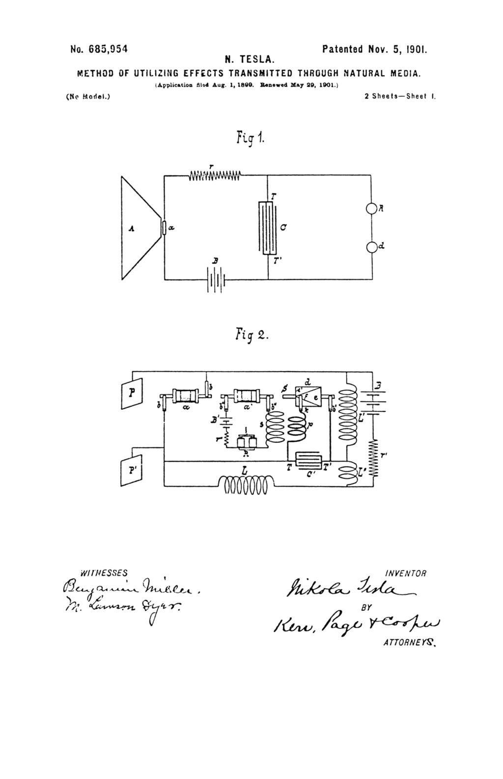
Assuming that the disturbances [the RF signals] which are to be investigated or utilized for some practical end, are rays identical with, or resembling ordinary light, the sensitive device a may be a selenium cell [He’s arguing by analogy; he’s not really going to detect RF with a photocell, but the action will be analogous so that the patent examiner (and “those skilled in the art”) can understand] properly prepared so as to be highly susceptible to the influences of the rays, the ‘action of which should be intensified by the action of a reflector A shown in the drawing. [In the Diary drawings, he will use an antenna.] It is well known that when the cells of this kind are exposed to such rays of greatly varying intensity, they undergo corresponding modifications of their electrical resistance [he is describing an RF variable resistor], but in the ways they have been heretofore used, they have been of limited utility. [32,33]

Interestingly, in spite of the fact that his “Method” patent application was filed in August, 1899, he held off on his “Apparatus” patent application until November of that year. It is the apparatus to which we now turn.

Part III. Tesla’s Colorado Springs Receiver Research

In the course of my investigations of terrestrial electrical disturbances in Colorado, I employed a receiver, the sensitiveness of which is virtually unlimited. [34]

1. Receiver Architecture

In this section, we want to go into the Colorado Springs Notes and into the receiver patents filed in 1899 and see how Tesla explained the physical operation of his receivers. We will look closely at the circuit philosophy and its relation to subsequent developments in radio technology. In part IV we will explore the actual operation of specific radios that Tesla built and operated at Colorado Springs.

Starting with the receivers of June 29t' and July 1, 1899 (they are link coupled to a signal generator) we can see the variations in receiver circuit configurations which Tesla is testing. The notes clearly document his struggle for RF sensitivity. He starts by allowing the DC through the coherer to charge a condenser. The greater the RF present, the faster the condenser would charge.

(That’s right, because of the non-linear resistance of the coherer the time constant depends upon the RF field strength.)

Furthermore, and this is important, the receiver responds only to the leading edge of the incident electrical disturbance. It is like a sampling scope which is triggered when the incident wave packet is above a given threshold voltage; and then remains on, sampling the signal for only a brief duration (typically a few hundred microseconds), pouring DC from a local battery into a storage capacitor, and then it turns off and remains so until the ‘sensitive device’ is decohered and is again ready to detect the presence of an RF signal. This windowing process is almost like a ‘delayed range gate’ operation in a radar receiver. (This manner of operation may account for some unusual actions.)

2. The Condenser Method of Magnifying Effects

On June 29, 1899 Tesla refers to a receiver “condenser method”, for which a patent application was being filed through the Curtis law firm. On July 1, 1899 he calls it the “condenser Method of Magnifying effects”. We take it that this receiver is the one employed in the famous July 3`a lightning-standing wave discovery. The circuit operation is explained, not in the Diary, but in US Patents #685,954 (Method: application filed August 1, 1899) and #685,956 (Apparatus: application filed November 1, 1899).

The technique, shown in Figure 9 (Fig. 1), uses the incoming RF to “turn on” a uniformly rotating coherer, which is in series with a DC battery and a substantial storage capacitor (about 1/2 Current flows [with time constant (r+-R. OC)]) charging the condenser until the rotating coherer decoheres, leaving a small charge on C. The energy (from the RF controlled battery) is accumulated over many, many coherer pulses in the storage condenser. This process is continued to the point that the battery supplies sufficient energy to the condenser to be able to “operate a receiving device R” or to “discharge through a transformer” and “operate a receiver by the currents so developed in the secondary of the transformer”. The ‘make/break’ device d, shown in Tesla’s figure, served to “periodically discharge the condenser C through the sensitive receiver [earphone] R”.

The ‘receiving device R’ could be a sensitive relay, an earphone, a Morse inker or a Morse sounder. None of these devices had the sensitivity or capability to respond to the RF and, with the possible exception of the earphone, none could respond to a simple envelope detector tracking the RE Clearly, the process involved repeated (almost uniform) sampling of the RF envelope (actually sample-and-hold) with baseband low pass filtering. By this method, Tesla’s apparatus could gain an order of magnitude advantage over the use of the coherer alone. But he wasn’t satisfied. He proceeds to squeeze even more performance from the detector.

3. Multiple Coherer Operation

He goes on to use the charge on the condenser to discharge into a coupled coil and allow the new RF oscillations to bias another coherer to a lower DC resistance point than the first coherer. The second coherer was used to trigger a fine telegraph relay (which Tesla designates as ‘the receiver - R’).

In trying to reconstruct Tesla’s multi-coherer circuits, we found it very difficult to get the decohering to work in unison. From the many variations in the Diary it is obvious that Tesla also ran into similar problems. (See July 21, 22, 28, 1899.)

Tesla also found that he could use parallel tank circuits to cause the RF voltage from an antenna to rise, causing the first coherer to act more favorable. This is not unlike the quarter-wave technique used in the Slaby-Arco arrangement, where the coherer was positioned to be at the point of a voltage maximum.

4. “The Self-Exciting Process”

While he was struggling with the receivers, he was also working on his ‘magnifying transmitter’. We speculate that the term ‘magnifier’ [35] caused him to employ the use of the resonator in his receivers. The resonator clearly gives a sharp rise in the RF voltage derived from the signal.

Using the coherer in the generation of RF oscillations, via a large capacitor and small inductor, must have taken him back a few years to the invention of the original version of the coil bearing his name. With some clever thinking, Tesla developed a circuit that would take a very small RF signal and cause a condenser to charge to a point and then discharge into the primary of a coil. He had to use a small clock driven mechanical break (switch) for this.

The new RF oscillations were coupled into a resonator (the secondary), and the resonant rise on the latter was impressed (via feedback) back across the coherer. (He didn’t need the two separate coherers.) This, in turn, would further reduce the DC resistance of the coherer, causing the condenser to charge to even a higher level. The next discharge into the primary coil causes a higher output from the resonator, and the DC resistance from the coherer drops even further. This process will continue until the original RF signal is removed or the coherer reaches its minimum DC resistance.

Tesla called this the “self-exciting” process, and it was one of the most important of his Colorado Springs discoveries. (See August 3, 1899.) On August 11, 1899 Tesla even uses the tapped-resonator version of Tesla coil (mistakenly called an ‘Oudin coil’ in the popular literature of today) instead of the link coupled version in his receiver.

The feedback self-exciting operation causes the sensitivity of the receiver to be greatly increased, even further than the “condenser Method of Magnification”. The sensitivity is now dependent only on the charging time constant as manifested through the slope of the graph, i.e. the material used to make the filings in the coherer.

5. Receiver Sensitivity

Experimenting with the materials mentioned in the Diary, we found that nickel seemed to work the easiest. The smallest detectable RF signals in our crude receivers were on the order of 80 millivolts peak-to-peak. Compare this value to other receivers without feedback. Experimentally, we found this to be in the 10 to 80 volt peak-to-peak range. By today’s standards a 100 mV sensitivity is not much, of course. (With careful experimentation these numbers might have been reduced by, perhaps, an order of magnitude.) But, for 1899, this was quite remarkable. Tesla did not patent this method as regeneration, nor as feedback, but as increased sensitivity by the “condenser method of magnification”.

6. Receiver Selectivity

We have said much about the sensitivity of his receivers, but what about the selectivity (i.e., Q or bandwidth)? Tesla’s feedback system was based on a resonator at the same frequency as the RF being detected. Since it is known that the resonator is an extremely high Q device, one must believe that the receiver was very selective. Experimentally, we found this to be true. It is this fact that makes the receiver cumbersome.

The tuning of the receiver is dependent on the frequency of the resonator. Changing the frequency, or tuning the receiver, meant removing or adding turns of wire to the resonator. Later in the Diary, Tesla is seen making the receiver have interchangeable resonators much like the plug-in coils that were so popular in communication receivers thirty years later. (The authors still have a fondness for National’s HRO receivers.)

7. Comparison to Heterodyne and Regenerative Receivers

Credit for the invention of the regenerative receiver should be given to Edwin Armstrong. He received the IEE’s first Medal of Honor, in 1917, for its creation. However, recognition should be extended to Nikola Tesla since, clearly, he was the first one in history to employ feedback in a circuit to improve the sensitivity of a receiver.

The first “beat” receiver for RF was invented by Nikola Tesla in the early 1890’s. [36,37] Tesla’s foreshadowing of the heterodyne receiver is really an untold story in electrical history. He used locally generated RF oscillations and an iron wire driven by antenna currents in a ‘magnetic detector’ stage. The wire, whose tension could be varied, was part of a tuned circuit and it was suspended through a constant magnetic field. (The physics is similar to that employed by Mahlon Loomis.) The mixing took place in the nonlinearities of the iron wire (the effect “discovered” by Barkhausen in 1918), and audible beats were easily heard (the mechanically oscillating wire was also a “speaker”).

“When the frequencies were very high, I combined two frequencies very nearly alike. That gave me a low beat... I used machines of this character from 1892.” [38]

By 1897, Tesla had already used this heterodyne receiver at West Point to listen to his transmitter 30 miles away at his New York City laboratory on Houston Street. In the following discussion, we know that he is referring to such men as Lord Kelvin and Hermann von Helmholtz, who both visited Tesla’s laboratory.

Counsel: Did you hear it?

Tesla: You could hear it all over the place.

Counsel: You mean you didn’t have to have your ear in the phone to hear it?

Tesla: o, not at all.

Counsel: Was there anything hidden about these uses, or were they open so that anyone could hear them?

Tesla: There were thousands of people, distinguished men of all kinds, from kings and [the] greatest artists and scientists in the world, down to old chums of mine -- mechanics, to whom my laboratory was always open. I showed it to everybody; I talked freely about it. [39]

The heterodyne principle, however, is commonly attributed in books on the history of technology to Reginald Aubrey Fessenden. [How do these things attain perpetuity? Who has been writing our electrical technology history books?!!] In Greek, heterodyne means to mix two different forces, and Fessenden coined the term. It is derived from ετερος meaning the other of two, and δυναμς meaning miraculous power (dyne = force).

Fessenden needed a detector appropriate for CW reception. He reasoned, in late 1901 (almost a decade after Tesla had already built and demonstrated the principle), that if the antenna current and a locally generated RF signal were both fed directly to an earphone, one could hear the beat frequencies, which could be made to occur at audible rates. [40] It turned out that, fortuitously, because of the nonlinearities of the magnetic earpiece (which functioned as a mixer stage - just as Tesla had been using!), one could indeed “hear” Fessenden’s heterodyne beat.

But, Fessenden took out the patent and gave it the heterodyne name, and his recognition has stuck - at least among authors and journalists in the “history of technology” community.

Regeneration is the process of supplying energy to a circuit to reinforce the oscillations existing in it. A workable technique for regeneration (RF feedback) by self-heterodyning is commonly traced to the September 22, 1912 third story bedroom discovery of Edwin Howard Armstrong (1890-1954). (There is a marvelous interview with Armstrong’s niece in the Ken Burns PBS documentary “Empire of the Air”, based on the 1991 HarperCollins book of the same title by Tom Lewis.)

In 1917 Armstrong published a masterful engineering study of the regeneration phenomenon. [41] At that time, the vacuum triode was thought to be an ‘electron relay’ between the input (grid circuit) and output (plate circuit). In retrospect, the three types of RF amplifying action that can occur in an “electron relay” may be identified as follows:

1. Fritz Lowenstein (Tesla’s assistant at Colorado Springs and first Vice-President of the IRE) found that he could obtain linear (now called Class A) amplification from a grid biased audion. [42]

2. Lee De Forest realized that he could actually make CW oscillations by using unity gain audion feedback.

Amazingly, he could never really explain the circuit analysis. De Forest earned a PhD under J. Willard Gibbs at Yale and, knowing that heated gases could detect RF, his formal training lead him to attempt to force the physics of triodes into the realm of the kinetic theory of gases. The name audion was coined by De Forest’s assistant as a contraction of the terms audio (Latin) detector and ion (Greek) controller. They thought that “ionization” was critical to the triode’s operation. [43]

The following quotes reflect this line of thought...

I think it [the operation of the audion] is due to the ionization of the residual gases... The gas particles are the carriers. (De Forest, October 1906 lecture to the AIEE.)

A careful study by others would soon lead to the understanding that “...none of the methods of producing amplification or oscillation depend on a critical gas action.” (Armstrong, March 1915, lecture to the IRE)

But, it was a youthful electrical engineering college senior that astonished the industry.

3. Armstrong discovered that RF feedback [44] of a received signal, coupled from a single-stage plate circuit back to the grid circuit, would make an extremely weak received carrier signal grow in amplitude virtually to the point of overload distortion.

(The high frequency component serves for RF amplification of the signal in Armstrong’s remarkable receiver circuit.) [45] While voltage gains of 35 dB could be attained from tubes operating Class A, Armstrong’s approach gave RF gains in excess of 74 dB with the available tubes of that day!

Is a triode, or three element device, required for this process? No. The overall process of regeneration is equivalent to injecting a signal into a tuned tank circuit in which a negative resistance has been inserted. (Feedback amplification is the mechanism by which negative resistance arises in Armstrong’s embodiment.) The result is to neutralize the positive (loss) resistance of the tank. Not only does the amplitude of the RF signal grow (the amplification is limited by the tube breaking into oscillation), but the Q multiplies as the total loss decreases (ω_ο/2α). A similar result can be obtained with any negative resistance device today, such as a tunnel diode or a parametric amplifier. These are two terminal devices.

In the discussion correspondence following Armstrong’s 1917 regeneration paper, Carl Ort [46] provided further insight on heterodyne receivers. Ort points out that instead of using an ‘electromagnetic receiver’, as was employed by Fessenden, he and his colleagues used an ‘electrostatic receiver’ (coherer) and found that these could be made “very sensitive” by local oscillator RF injection. [47,48] (This is not the superheterodyne principal. [49] That was not to be discovered for several years yet to come, while Armstrong was serving in France during WWI.)

Apparently, IRE Vice-President J.V.L. Hogan replaced the ‘electro-static receiver’ by a crystal detector “with the result that much higher sensitiveness could be obtained than with any previous receiver.” [50,51,52] (Those crystal set experimenters in our midst that desire increased sensitivity should try this out.) However, according to Ort’s 1917 remarks the reason for the great gain was never understood until Armstrong’s landmark regeneration investigation.

Mr. Armstrong’s experiments have shed new light on these phenomena and have indicated that the amplification obtained with a rectifying detector depends on the energy of the local oscillations which are applied to the detector, and that while the energy received is not magnified at all, the sensitiveness of the detector is increased. This increase is independent of the frequency of oscillation of the local source. [53]

This is exactly as Tesla described, 18 years earlier, in his 1899 Colorado Springs Notes! The increased sensitivity is due, as reported in our experiments above, to the steeper slope. Clearly, this is the very phenomenon discovered and embodied in the sensitive receivers shown in Tesla’s Diary.

Ort continued his comments with a personal experience, that occurred in Austria in December of 1912, in which a remarkable gain was obtained from a simple detector.

I investigated the phenomenon, applying sustained oscillations directly to the detector and found that the amplification was due to the increase of sensitiveness of the detector. Every... rectifying detector showed this characteristic. I found that the amplification could be obtained with any frequency not audible to the human ear. The limit of amplification was determined by the maximum impressed voltage of sustained RF at which the detector burned out. I was able to obtain amplifications of about 2000 (66 dB).”

Again, we recognize Tesla’s pioneering and priority in the development of sensitive RF detection.

8. Armstrong’s Superregenerator Detectors

In connection with Armstrong’s regenerator work, subsequent to WWI, we should mention, in passing, the term ‘Superregeneration’. The ‘Superregenerative Receiver’ was introduced by Armstrong in 1922. [54,55] These receivers are extremely sensitive, going right down to the thermal noise floor, and as such were not only of considerable benefit historically, but are still of interest today. [56] Stockman has pointed out that,

Superregeneration is the condition in a regenerative system that produces a growing transient of oscillation, prevented from becoming a sustained oscillation by means of a repeated quenching action. [57]

Armstrong, in his pioneering publication on superregeneration, had described his discovery that if one can obtain a periodic variation between the negative and positive resistance in a tank circuit, then two important things will happen. First, during those intervals when the negative resistance is greater than the loss resistance, the circuit will produce great amplification of an impressed emf - a growing transient response. And secondly, the alternations in resistance will prevent the circuit from becoming self excited to the extreme.

Armstrong was able to report that the voltage gains obtainable with superregeneration were 10 to 20 times greater than he had been able to attain with standard regeneration. While an exceedingly thorough engineering analyses was carried out by HA. Wheeler, (“) the most readable account still seems to be the old discussion due to Lauer and Brown. [59]

Part IV. Colorado Springs Receiver Operation

We next turn to the receivers of the Colorado Springs Notes. In the Diary, on page 110 (July 29, 1899), Tesla gives the speed of rotation of the coherers as “about 24 per minute” and the break speed as “72 per second”. He also tells us that the coherer resistance was “over 1,000,000 ohms, but when excited the resistance fell almost exactly to 50 ohms.”

There are many, many circuit configurations in the diary. Figure 10, from August 3, 1899 shows Tesla’s use of feedback. Consider the receiver of September 1, 1899 shown in Figure 11, and re-drawn in Figure 12. Notice the position of the coherer at the high voltage point on the resonator-secondary. The final receiver recorded in the Diary is discussed on Sunday, September 17, 1899, and is shown in Figure 13.

1. Architecture

Again, the circuit is deceptively simple! First, notice the architecture. There are four superimposed circuits in the schematic drawing of Figure 12:

A. The C_p charging circuit. B₁ charges C_p through resistance r with time constant ti, = rC,. This places a DC voltage on C_p. For reasons which will soon be evident, this will be called the “Sensitivity Control”.

B. The “Lumped Coupled Coils” (1891 version of a Tesla coil) consisting of C_pL_p, L_s (and its associated self-capacitance C_s), and break d. This is a local RF oscillator, but its application is somewhat different than the LO for mixer injection taking place in Armstrong’s Superheterodyne receiver. Tesla’s LO generates a high voltage RF potential (on the order of several hundred volts) to impress upon the coherer device “a”. Note the position of “a” at the top of the secondary coil. The bottom of the secondary coil is grounded. The importance of this cannot be stressed enough. When the coherer’s resistance is high (~1MΩ) its presence will not impact the operation of the LO circuit.

C. A baseband detector stage, which operates while the break device (d) is closed. This consists of the coherer “a”, the primary capacitor C_p, the secondary coil L_s (which at baseband behaves as a low impedance resistance ~50Ω for a DC return path for battery B through the coherer “a”), and the indicators R (a 900? DC relay or telegraph indicator) and the circle (a high impedance earphone) both of which are battery driven. The coil L is an RF choke to provide a high impedance to any RF in the detector stage.

D. The antenna-ground circuit which provides the input RF signal. This circuit consists of the antenna capacitance Cp the coherer device “a”, the resonator coil L_s, and the ground connection, which is most important. When there is no RF signal between C’ and ground, the coherer resistance is high (~1MΩ).

When an RF signal of sufficient strength is present, the coherer resistance drops considerably (ultimately to about 50Ω).

As mentioned above, the sensitivity of a classical coherer was known to be quite poor, requiring signal levels on the order of tens of volts in Figures 3 and 6. Both Tesla and Lodge placed the coherer in a tuned circuit (Figure 2) which not only raised the RF voltage across the coherer (by resonant rise), but also provided selectivity.

Tesla’s use of this circuit can be documented since it was part of the 1898 Patent Application for his radio controlled “telautomaton”, or robot. However, Tesla had discovered something new, which greatly increased the sensitivity of the coherer - and that was the injection of RF into the coherer.

There is a surprising amount of discussion concerning the construction, physics, and operation of coherers in Tesla’s US Patents:

#613,809 (Filed: July 1, 1898; Issued: Nov. 8, 1898)
#685,954 (Filed: Aug. 1. 1899; Issued: Nov. 5, 1901)
#685,956 (Filed: Nov. 2, 1899; Issued: Nov. 5, 1901)

2. Operation

We think that the receiver operates as follows:

1. The B₁r circuit charges C_p (which controls the amount of RF energy which the oscillator impresses on the coherer). As a result, r sets how much RF is generated locally in the receiver and the sensitivity point of the coherer, i.e. - its DC resistance.

Further, it controls the time constant on C_p, which is desired to be huge with respect to the make/break of the switching device d. The resistor “r” is the receiver’s “Sensitivity” control. Typically, r ≈100kΩ and Cp≈0.1-0.5µF. This would give τ≈10-50 ms.

2. An RF signal in the ground end of the resonator (secondary) is stepped up by the VSWR (Q for lumped coils). Enough RF is desired to take the device to the knee of its characteristic curve.

3. The two RF voltages together are sufficient to lower the DC resistance of the coherer by a very small amount (1Ω M drops to say 900 kΩ).

4. The DC resistance now being somewhat less means that Cp can charge to a portion of the voltage on battery B.

5. When “d” closes C_p and L_p will produce a large RF out of the resonator L_s further reducing the DC resistance of “a” (say, going from 900 kΩ down to 500Ω).

6. This allows C_p to charge to a larger portion of B, which will make the output of the resonator rise even further, and the coherer’s DC resistance will drop dramatically (say, down to 1000 Ω).

7. This process repeats successively until the coherer resistance drops low enough (about 50Ω) for the telegraph clicker to click.

The RF signal initiated the process, but after its expiration the device continued to avalanche until a click registered.

8. Nothing more will (or can) happen until the device is decohered (shaken) back to 1 MΩ.

The problem with a CW carrier is that the continuously present RF keeps the coherer DC resistance at 50Ω. Consequently, coherers work best for pulsed signals. The coherer is really a detector which says RF yes, or RF no. Our experiments indicated a 60 dB improvement in sensitivity when we used the same coherer and went from Branly’s mode of operation to Tesla’s.

3. Receiver Construction

We re-fabricated the receiver more-or-less to the specifications given by Tesla. The measured parameters for the reconstructed receiver of Figure 11 were as follows:

C_p = 0.1µF*          Cs = 50 pF
L_p = 500µH           Ls = 1000 mH
R_p = 1 S2,              Rs= 600 S2
Q_p = 72.3              Qs = 235
M = 450 µH           Vo = 10 V
k = 0.0201             k, = 0.0077
fP = 22.5 kHz         f_s = 22.5 kHz
R_Coh = 1 MΩ (open) and 50 Ω (closed)
B₁ = 9 V                 B = 1.5 V

*Tesla used 1/2µF

Our “break” device was a TTL driven micro-relay running at 72 BPS (the same rate as Tesla’s clockwork driven break, see CSN pg. 110) with about a 1000µs duration. Tesla placed the portable receivers in two boxes 9”x 10”x 14”. His “synchronized coils” were wound on a form 10” diameter by 48” high and 24” diameter by 18” high supported on a photographic tripod (CSN, pp 187-188).

4. TCTUTOR Analysis of the Local Oscillator

Our TCTUTOR manual gives a thorough mathematical analysis of lumped coupled coils (as well as distributed resonators), and the “Master Oscillator” section of the software program is appropriate for analyzing the coupled tuned oscillators in Tesla’s receivers. Using this tool along with the physically constructed operational receiver from the Colorado Springs Notes, we have obtained some rather surprising results.

We think that we too have heard the “Martian signals” and can finally resolve this puzzling issue. [At the 1994 International Tesla Symposium we played a tape recording of the receiver detector output, which definitely is a signal characterized by “a regular repetition of the numbers one, two, three ...”. [60,61,62,63] This was probably the first time that anyone has heard the “Martian signals” since Tesla and Lord Kelvin, and was certainly their first public exhibition.] The signals were also highlighted in his Colorado Springs Notes December 8, 1899 entry and Tesla’s Letter to the American Red Cross dated “Christmas, 1900”, which for Tesla would have been January 7, 1900 - the date of the last entry in the Diary and of Tesla’s departure from Colorado Springs.

The TCTUTOR computer nun gives a “double humped” spectrum, with spectral peaks at 22.3 kHz and 22.7 kHz (as would be expected with such tight coupling). The voltage across the second capacitor, V_C2(t), is especially interesting. It is a double side-band signal with an effective “carrier” at about 22.5 kHz and a “beat” period of 2500 [ts, which corresponds to a frequency of 400 “beats per second”]. (See Figures 14 and 15.) Interestingly, the envelope of V_C2(t) is maximum at about t = 900 µs, where V_C2 ≈ 25xV_o. The 400 beats per second was of interest and it could be heard in audio pulses with the earphones in the manner (inappropriately) attributed to Fessenden.

V. Summary

There are three modes of operation for coherer receivers:

1. Branly’s mode - in which the coherer DC resistance collapses from a megohm to a few ohms when an RF signal exceeds the knee in the i-v characteristic.
2. Lodge’s mode - for which the coherer crudely behaves as an analog envelope detector.
3. Tesla’s RF feedback exploitation of the voltage-controlled resistance of the coherer.

In modes 1 and 3 coherer agitation is required to decohere the device between pulses, and the detector does not function for CW. Mode 2, instead of mechanical decohering, requires extreme mechanical stability. Sharp chips work best for the envelope detector mode of Lodge (which simulates today’s crystal sets). Fine particles work best to get the go/no-go, steep-kneed, RF detector curves of Branly. [But, either a strong signal is required to get operation at the knee (as Branly did), or a large bias is needed to get operation out at the knee.]

Tesla discovered a technique by which the nonlinear resistance of a coherer (as a function of injected locally generated RF) could be triggered and exploited by an exterior pulse signal. Having a weak signal initiate the injection of high voltage RF, and using the resulting (voltage controlled) resistance decrease to “ratchet up” the Local Oscillator RF (an 1891 lumped coupled coils version of his Tesla coil), which further decreased down the coherer resistance (the process repeating over and over) so that ultimately the relay would be triggered, gave Tesla at least a 60 dB improvement in sensitivity over contemporary (1899) receiver technology. It was not until Armstrong’s discovery of regeneration (US Patent # 1,113,149) that receivers could be made more sensitive than this.

References

1. Delaval, E., Philos. Trans. Roy. Soc. London, Vol. 51, Pt. 1, 1759, pp. 83-88.
2. Kryzhanovskii, L.N., “The Coherer: Preparing the Way for Wireless,” Electronics World + Wireless World, March, 1992, pp. 212-214.
3. Munck, P.S., “Versuche uber die Fahigkeit starrer Korper zur Leitug der Elektricitat,” Annalen der Physik und Chemie, Vol. 34,1835, pp. 437-463.
4. Branly, E., Compt. Rend., Vol. 111, 1890, p. 785; Vol. 112, 1891, p. 90.
5. Lodge, O., Journal IEE, Vol 19, 1890, p. 346
6. Lodge, O., Nature, Vol 50, 1894, pp 133-139
7. Susskind, C., “TEarly History of Electronics - Pt III”, IEEE Spectrum, Apr, 1969, pp 69-74
8. Kryzhanovskii, LN, “A History of the Invention of and Research on the Coherer,” Soviet Phys Uspekhi, Vol 35 No 4, Apr 1992, pp 334-338
9. KryzImovskii, L.N., “A History of the Invention of and Research on the Coherer,” Soviet Physics Uspekhi, Vol. 35, No. 4, April, 1992, pp. 334-338.
10. Philips, V.J., “Early Radio Wave Detectors,” Peter Peregrinus Press, 1980, Chapter 3.
11. Kryzhanovskii, L.N., “Coherer Anomaly,” Electronics World + Wireless World, July 1992, pg. 607.
12. Lodge, O., Phil. Mag., Vol. 37, 1894, p. 94
13. Lodge, O., Electrician, Vol 40,1898, p 87
14. Lodge, O., Proceedings of the Royal lnst, Vol. 16, 1902, p. 72
15. Auerbach, F., Annalen der Physik und Chemie, Vol. 64, 1898, p. 611.
16. Branly, E., Lumiere Electrique, Vol. 40, 1891, p. 506.
17. Branly, E., Compt. Rend, Vol 112, 1891, p 90; Vol. 118, 1894, p 348; Vol. 125, 1897, p. 163
18. Branly, E., Bull. Soc. Sci, Franc. Phys., 1897, p.135.
19. Branly, E., Cong. Internat Physique, Vol. 2, 1900, p. 325.
20. Ginden, L.G., and AE. Vol’pyan, “Structure Formation in Disperse Systems in and Electric Field,”, Russian Chemical Reviews (Uspekhi Khimi), Vol. 37, No. 1, 1968, pp. 53-60.
21. Kryzahnovskii, Uspekhi, 1992, loc cit.
22. Aitken, H.G.J., S3ntony and Spark: The Origins of Radio, Princeton University Press, 1985, pg. 248.
23. von Arco, Dr. Georg G. (Count), Telefunken letter to Tesla, June 2,1931. (See Tribute To Nikola Tesla, V. Popovic, editor, Nikola Tesla Museum, Beograd, 1961, pp. LS:28-29.)
24. Corum, J.L., K.L. Corum, and J.F Corum, “Mahlon Loomis: Terra Alta’s Neglected Discoverer of RF Communication”, Proceedings of the 1992 International Tesla Society Symposium, Colorado Springs, Colorado.
25. Marconi, G., “Magnetic Detector”, British Patent #10,245; 1902.
26. De Forest, L., “Magnetic Detector”, US Patent #772,878, Filed June 20, 1903; Issued October 18, 1904.
27. De Forest, L., “Art of Duplex Wireless Telegraphy”, US Patent #772,879, Filed June 4, 1903; Issued October 18, 1904.
28. Loomis, MT., Radio Theory and Operating, Loomis Publishing, Washington, DC, 1930.
29. Appleby, T., Mahlon Loomis. Inventor of Radio, 1967, 164 pp.
30. Anderson, L.L, Nikola Tesla: On His Work With Alternating Currents, Sun Publishing, Denver, 1992, pg. 27.
31. Tesla, Nikola, “Method of and Apparatus for Controlling Mechanism of Moving Vessels or Vehicles”, US Patent #613,809; Filed: July 1, 1898; Issued November 8, 1898.
32. Tesla, Nikola, “Method of Utilizing Effects Transmitted Through Natural Media”, US Patent #685,954, Filed August 1, 1899; Issued November 5, 1901. See Dr. Nikola Tesla Selected patent Wrappers, compiled by J.T. Ratzlaff, Tesla Book Company, 1980, Vol. II, pp. 404-454.
33. Tesla, Nikola, “Apparatus for Utilizing Effects Transmitted Through Natural Media”, US Patent #685,956, Filed Nov 2, 1899; Issued Nov 5, 1901. See Dr. Nikola Tesla. Selected patent Wrappers, compiled by J.T. Ratzlaff, Tesla Book Co, 1980, Vol. III, pp. 455-494.
34. Tesla, Nikola, “Signals to Mars Based on Hope of Life on Planet, New York Herald, October 12, 1919, Magazine Section.
35. Corum, K.L. and J.F. Corum, “Tesla and the Magnifying Transmitter,” Proceedings of the 1992 Int’l Tesla Symposium, Colo Spgs, CO.
36. Anderson, L.L, Tesla: On His Work With Alternating Currents, Sun Publishing, Denver, 1992, pp. 23-29.
37. Cohen, S., “Dr. Nikola Tesla and His Achievements”, The Electrical Experimenter, February, 1917, pp. 712-713, 777.
38. Anderson, L.L, Nikola Tesla: On His Work With Alternating Currents, Sun Publishing, Denver, 1992, pg. 24.
39. Anderson, L.L, Nikola Tesla: On His Work With Alternating Currents, Sun Publishing, Denver, 1992, pg. 29.
40. Fessenden, RA, US Patents #706,740 (Filed: Sept 28, 1901; Issued: August 12, 1902) and #1,050,728.
41. Armstrong, E.H., “A Study of Heterodyne Amplification by the Electron Relay”, Proceedings of the IRE, Vol. 5, 1917, pp. 146-168.
42. Lowenstein, F, US Patent #1,231,764. Filed: 1912; Issued 1917.
43. De Forest, L., “The Audion: A New Receiver for Wireless Telegraphy,” AIEE Transactions, Vol. 25, 1906, pp. 735-779. (See pp. 769 and 778.)
44. Armstrong, E.H, (Regeneration Feedback Invention), US Patent 41,113,149. Filed: October 29, 1913; Issued: 1914. This is the famous patent that Armstrong flew on a flag for De Forest to see from his home.
45. Lauer, H, and H Brown, Radio Engineering Principles, McGraw-Hill, 1928, pg. 225.
46. Ort, C., “Discussion”, Proceedings of the IRE, Vol. 5, 1917, pp. 163-166.
47. Ort, C. Elektrotechnische Zeitschrift, 1909, pg. 655.
48. Ort, C., Archive fur Elektrotechnik, Vol 1, 1912, pg. 192.
49. Armstrong, E.H., (Superheterodyne Receiver), US Patent #1,342,885. Filed: February 8,1919; Issued: June 8, 1920.
50. Ort, C., “Discussion”, Proceedings of the IRE, Vol. 5, 1917, pp. 163-166.
51. Hogan, J.L., and Lee, Proceedings of the IRE, Vol. 1, July, 1913; and US Patent 1,141,717.
52. Liebowitz, B., Proceedings of the IRE, 1915, pg. 185.
53. Ort, C., “Discussion”, Proceedings of the IRE, Vol. 5, 1917, pp. 163-166.
54. Armstrong, E.H, “Superregenerative Receiver, 1922, US Patent #1,424,065. For this patent, David Sarnoff paid Armstrong $200,000 and 60,000 shares of RCA stock on June 30, 1922.
55. Armstrong, E.H, “Some Recent Developments of Regenerative Circuits”, Proceedings of the IRE, Vol. 10, 1922, pp. 244-260.
56. Kitchin, C., “The Lost Art of Regeneration”, Electronics Now, March, 1994, pp. 66-73, 80, 86-87.
57. Stockman, FL, “Superregenerative Circuit Applications”, Electronics, February 1948, pp. 81-83.
58. Wheeler, H.A., Wheeler Monographs, Vol. 1, No. 3, 1948, pp. 1-46, “A Simple Theory and Design Formulas for Superregenerative Receivers”; Vol. 1, No. 7, 1948, pp. 1-30, “Superselectivity in a Superregenerative Receiver”.
59. Lauer, FL, and FL Brown, Radio Engineering Principles, McGraw-Hill, 1928, pp. 225-235.
60. Tesla, Nikola, “Talking with Planets,” Collier’s Weekly, February 9, 1901, pp. 4-5.
61. Tesla, N., “Talking With Planets,” reprinted in PolXphase Electric Currents, Chapter XIV of Volume 4 of The Library of Electrical Science, S.P. Thompson, Ed., Collier & Son, NY, 1902, pp. 225-235.
62. Tesla, Nikola, “Signals to Mars Based on Hope of Life on Planet,” New York Herald, October 12, 1919, Magazine section. Reprinted in Tesla Said, complied by J.T. Ratzlaff, Tesla Book Company, 1984, pp. 219-221.
63. Tesla, Nikola, “Interplanetary Communication,” Electrical World, Sept 24, 1921, pg. 620.